

General introduction
With the advent of recent computer technology, the role of digital simulation has become predominant, as it can take advantage of the increase in computing resources and above all their parallelization. It is therefore increasingly used in the decision-making process, which means that it is no longer necessarily just descriptive, but must become increasingly predictive, by supporting the confidence that can be placed in its predictions in the finest possible way.
In this section, we will discuss a system 𝓢, whose design (dimensions, materials, initial conditions, ...) is characterised by a vector x ∈ X, and which we can attempt to model in different ways. The different levels of modelling thus introduce possible sources of uncertainty and bias, which are discussed later.
1. a mathematical model to describe perfectly certain variables of interest in the system (which we will call, for example, y(x) ∈ Y.
This model is not necessarily known or even attainable, but it describes "reality";
2. a parametric model ysim(-) describing as best as possible the same variables of interest in the system (this model not necessarily being equal to the previous level).The latter is normally representative of the understanding of the system and requires two types of parameters:
- the input parameters, simulated or measured,xξ ∈ Xin which are the factors on which the parametric model depends for each estimate (the vector ξ can be remplaced by xmes or xsim depending on whether the input parameters have been measured or simulated);
- the simulation parameters θ (also called model parameters), which are often constant parameters;
3. an algorithm capable of correctly calculating the parametric model, if possible without error, but sometimes also requiring dedicated parameters :
- the parameters that enable algorithms to converge numerically νnom;
4. measurements of the system's variables of interest (ymes);
These different levels can be represented schematically in 1)a) where the "reality" (in black) is more or less well described by the 3 other levels of abstraction: the ideal parametric model (in red), its implementation in the form of an algorithm (in blue) and the experimental measurements made (in green).
FIGURE 1 - (a) Schematic representation of the different levels of abstraction of the variables of interest in the system. (b) Relationship between the different levels of abstraction.
This vision gives rise to the VVUQ (Verification, Validation and Uncertainty Quantification) approach, in which a number of concepts need to be defined :
Validation : this stage attempts to control simulation uncertainties εsim := ytrue - ysim (•, θ, νnom)that could arise from oversimplifying the phenomenon. A validated model is not, however, a perfect model, as this validation can be carried out on specific quantities and/or in a well-defined field of use (often restricted, but sufficient). It is often summarised as "Solving the correct equation".
Verification : this stage attempts to control the uncertainties involved in implementing the numerical model εnum := ymod (•, θ) - ysim (•, θ, νnom) which could arise from a mesh convergence problem, a rounding problem in floating-point arithmetic, bugs, etc. It is often summarised as "Solve the equation correctly".
Calibration : this stage, which is necessary once validation and verification have been carried out, attempts to define the optimal value of the model parameters θ and to control the uncertainties associated εθ. In Figure 1b, it is integrated into the "Model validation (operational)" process, the latter including, in addition, the uncertainties associated with the choice of modelling the uncertainties of the input parameters.
Uncertainty propagation: this stage attempts to estimate the impact of uncertainties in the input parameters on the variables of interest and, more generally, on the quantities of interest (a quantity of interest is a numerical datum, generally statistical, representative of the distribution of the variable of interest: the mean, the standard deviation, a quantile, etc.).
Very often, in the probabilistic approach, it is common to consider that the (conceptual) validation of the model and its verification are done before considering doing a more advanced uncertainty quantification analysis.
The main steps discussed above and in the rest of this chapter are grouped together in Figure 2, which shows the definition of the problem, i.e. the process, the quantification of the sources of uncertainty, the propagation of uncertainties and the sensitivity analysis.
.
Random : also known as statistics in some fields, these uncertainties represent the natural variability of certain phenomena.
Epistemic : These uncertainties are generally more complex because they reflect a lack of knowledge about the specific values of certain parameters, or about the underlying physical laws.
Another characteristic that is sometimes discussed in terms of separating uncertainties is whether they are reducible or irreducible. Uncertainties belonging to the first category can be constrained by new data, while those belonging to the second category can no longer be contained. It is customary to say that epistemic uncertainties are reducible while random uncertainties are irreducible.
However, this distinction is not so clear-cut because it can depend on the point of view and the goals: uncertainty about the lifetime of a component, if it is provided to you, is to be considered as a random uncertainty, but if you are the manufacturer of the said component, you can choose to use it as such or to launch an R&D process to improve the manufacturing process and try to reduce it. The acceptable cost (economic, temporal, structural, etc.) of the reduction is often taken into account.
In this section, we will discuss a system 𝓢, whose design (dimensions, materials, initial conditions, ...) is characterised by a vector x ∈ X, and which we can attempt to model in different ways. The different levels of modelling thus introduce possible sources of uncertainty and bias, which are discussed later.
I. Overview of digital simulation
The predictive capacity of numerical simulation implies the definition of several levels of abstraction, not mutually exclusive, the aim of which is to describe reality as faithfully as possible:1. a mathematical model to describe perfectly certain variables of interest in the system (which we will call, for example, y(x) ∈ Y.
This model is not necessarily known or even attainable, but it describes "reality";
2. a parametric model ysim(-) describing as best as possible the same variables of interest in the system (this model not necessarily being equal to the previous level).The latter is normally representative of the understanding of the system and requires two types of parameters:
- the input parameters, simulated or measured,xξ ∈ Xin which are the factors on which the parametric model depends for each estimate (the vector ξ can be remplaced by xmes or xsim depending on whether the input parameters have been measured or simulated);
- the simulation parameters θ (also called model parameters), which are often constant parameters;
3. an algorithm capable of correctly calculating the parametric model, if possible without error, but sometimes also requiring dedicated parameters :
- the parameters that enable algorithms to converge numerically νnom;
4. measurements of the system's variables of interest (ymes);
These different levels can be represented schematically in 1)a) where the "reality" (in black) is more or less well described by the 3 other levels of abstraction: the ideal parametric model (in red), its implementation in the form of an algorithm (in blue) and the experimental measurements made (in green).
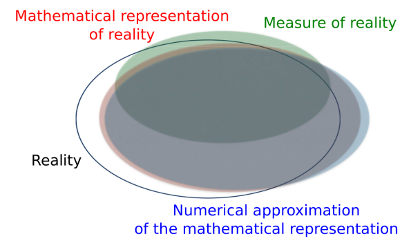
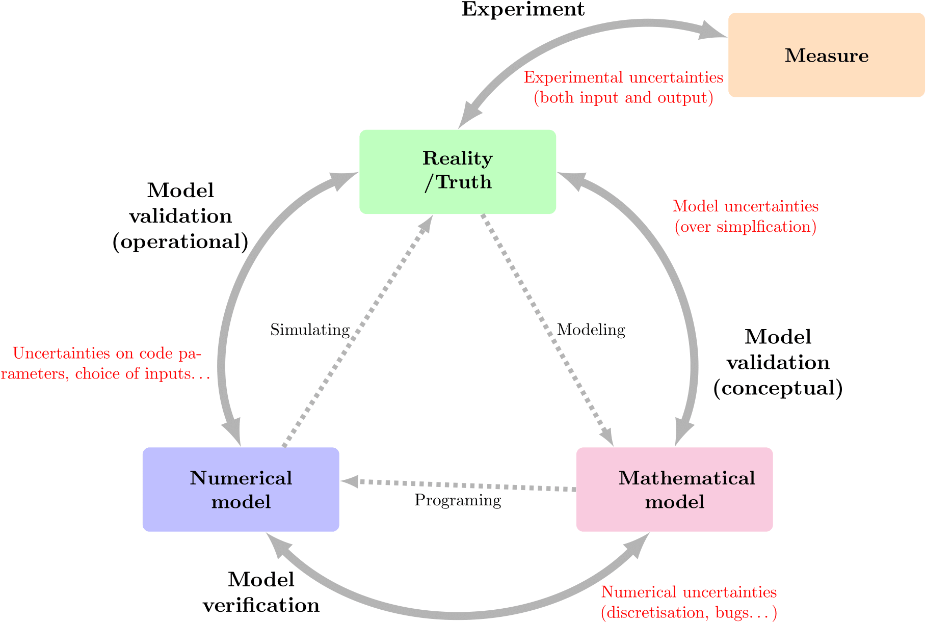
FIGURE 1 - (a) Schematic representation of the different levels of abstraction of the variables of interest in the system. (b) Relationship between the different levels of abstraction.
This vision gives rise to the VVUQ (Verification, Validation and Uncertainty Quantification) approach, in which a number of concepts need to be defined :
Validation : this stage attempts to control simulation uncertainties εsim := ytrue - ysim (•, θ, νnom)that could arise from oversimplifying the phenomenon. A validated model is not, however, a perfect model, as this validation can be carried out on specific quantities and/or in a well-defined field of use (often restricted, but sufficient). It is often summarised as "Solving the correct equation".
Verification : this stage attempts to control the uncertainties involved in implementing the numerical model εnum := ymod (•, θ) - ysim (•, θ, νnom) which could arise from a mesh convergence problem, a rounding problem in floating-point arithmetic, bugs, etc. It is often summarised as "Solve the equation correctly".
Calibration : this stage, which is necessary once validation and verification have been carried out, attempts to define the optimal value of the model parameters θ and to control the uncertainties associated εθ. In Figure 1b, it is integrated into the "Model validation (operational)" process, the latter including, in addition, the uncertainties associated with the choice of modelling the uncertainties of the input parameters.
Uncertainty propagation: this stage attempts to estimate the impact of uncertainties in the input parameters on the variables of interest and, more generally, on the quantities of interest (a quantity of interest is a numerical datum, generally statistical, representative of the distribution of the variable of interest: the mean, the standard deviation, a quantile, etc.).
Very often, in the probabilistic approach, it is common to consider that the (conceptual) validation of the model and its verification are done before considering doing a more advanced uncertainty quantification analysis.
The main steps discussed above and in the rest of this chapter are grouped together in Figure 2, which shows the definition of the problem, i.e. the process, the quantification of the sources of uncertainty, the propagation of uncertainties and the sensitivity analysis.
.
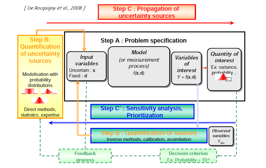
FIGURE 2 - Schematic representation of several stages in the VVUQ approach
II. Nature of uncertainties and modelling
Considering the propagation of uncertainties here (on the assumption that the model is conceptually validated and verified), it is interesting to ask questions about the properties of the uncertainties that we wish to take into account. The literature often discusses these by dividing their nature into two categories :Random : also known as statistics in some fields, these uncertainties represent the natural variability of certain phenomena.
Epistemic : These uncertainties are generally more complex because they reflect a lack of knowledge about the specific values of certain parameters, or about the underlying physical laws.
Another characteristic that is sometimes discussed in terms of separating uncertainties is whether they are reducible or irreducible. Uncertainties belonging to the first category can be constrained by new data, while those belonging to the second category can no longer be contained. It is customary to say that epistemic uncertainties are reducible while random uncertainties are irreducible.
However, this distinction is not so clear-cut because it can depend on the point of view and the goals: uncertainty about the lifetime of a component, if it is provided to you, is to be considered as a random uncertainty, but if you are the manufacturer of the said component, you can choose to use it as such or to launch an R&D process to improve the manufacturing process and try to reduce it. The acceptable cost (economic, temporal, structural, etc.) of the reduction is often taken into account.