

Documentation
/ Guide méthodologique
: 
| IV.2. The linear regression | ||
|---|---|---|
 | Chapter IV. Generating surrogate models |  |
When using the linear regression, one assumes that there is only one output variable and at least one input
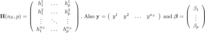
variable. The data from the training database are stored here in a matrix  where
where  is the number of elements in the set and
  is the number of input variables to be used. The idea is to
write any output as
is the number of input variables to be used. The idea is to
write any output as  , where
  are the regression coefficients and
  , are the regressors:
  simple functions depending on one or more input variables[7] that will be the new basis for the
linear regression. A classical simple case is to have
simple functions depending on one or more input variables[7] that will be the new basis for the
linear regression. A classical simple case is to have  and
and  .
.
The regressor matrix is then constructed as  and is filled with
In the case where the number of points () is greater than the number of input variables (), this estimation is just a minimisation of  which leads to the
general form of the solution
which leads to the
general form of the solution 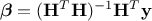 . From this, the estimated
values of the output from the regression are computed as
. From this, the estimated
values of the output from the regression are computed as  , if one calls
  .
.
As a result, a vector of parameters is computed and used to re-estimate the output parameter value. Few quality
criteria are also computed, such as  and the adjusted one
  . There is an interesting
interpretation of the
criteria, in the specific case of a linear regression, coming from the previously introduced matrix
. There is an interesting
interpretation of the
criteria, in the specific case of a linear regression, coming from the previously introduced matrix  , once considered as a projection
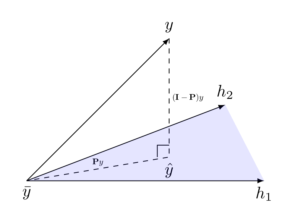
matrix. It is indeed symmetrical and the following relation holds
, once considered as a projection
matrix. It is indeed symmetrical and the following relation holds  , so the estimation
  by the linear regression is a orthogonal projection of
 onto the subspace
  spanned by the column of
 . This is depicted in
Figure IV.4 and it shows that the variance,
. This is depicted in
Figure IV.4 and it shows that the variance,  can be decomposed into its component explained by the
model
can be decomposed into its component explained by the
model  and the residual part,
  . From this, the formula in Equation IV.1 can be also
written
. From this, the formula in Equation IV.1 can be also
written 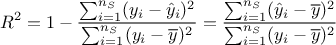
Figure IV.4. Schematical view of the projection of the original value from the code onto the subspace spanned by the column of H (in blue).
 |
For theoretical completeness, in most cases, the matrix is decomposed following a Singular Value Decomposition (SVD)
such as  . In this context
  and
and  are orthogonal matrices and
 is a diagonal matrix
(that can also be stored as a singular values vector
is a diagonal matrix
(that can also be stored as a singular values vector  ). The diagonal matrix always exists, assuming that the number of samples is greater
than the number of inputs (
). The diagonal matrix always exists, assuming that the number of samples is greater
than the number of inputs ( ). This has two main advantages the first one being that there is no matrix inversion to be performed,
which implies that this procedure is more robust. The second advantage is when considering the
). This has two main advantages the first one being that there is no matrix inversion to be performed,
which implies that this procedure is more robust. The second advantage is when considering the  matrix that links directly the output
variable and its estimation through the surrogate model: it can now simply be written as
matrix that links directly the output
variable and its estimation through the surrogate model: it can now simply be written as  . This is highly
practical once one knows that this matrix is used to compute the Leave-One-Out uncertainty, only considering its
diagonal component.
. This is highly
practical once one knows that this matrix is used to compute the Leave-One-Out uncertainty, only considering its
diagonal component.
| |  | |
| Chapter IV. Generating surrogate models |  | IV.3. Chaos polynomial expansion |