Documentation / Manuel utilisateur en C++ :

V.6. The kriging method

V.6. The kriging method
	Chapter V. The Modeler module

V.6. The kriging method

Warning

This surrogate model, as implemented in Uranie, requires the NLopt prerequisite (as discussed in Section I.1.2.2).

First developed for geostatistic needs, the kriging method, named after D. Krige and also called Gaussian Process method (denoted GP hereafter) is another way to construct a surrogate model. It recently became popular thanks to a series of interesting features:

it provides a prediction along with its uncertainty, which can then be used to plan the simulations and therefore improve the predictions of the surrogate model
it relies on relatively simple mathematical principle
some of its hyper-parameters can be estimated in a Bayesian fashion to take into account a priori knowledge.

Kriging is a family of interpolation methods developed in the 1970s for the mining industry [Matheron70]. It uses information about the "spatial" correlation between observations to make predictions with a confidence interval at new locations. In order to produce the prediction model, the main task is to produce a spatial correlation model. This is done by choosing a correlation function and search for its optimal set of parameters, based on a specific criterion.

The gpLib library [gpLib] provides tools to achieve this task. Based on the gaussian process properties of the kriging [bacho2013], the library proposes various optimisation criteria and parameter calculation methods to find the parameters of the correlation function and build the prediction model.

The present chapter describes the integration of the gpLib inside Uranie, and how to create a new kriging model and use it. We first give a quick reminder of what kriging is. Next, we describe how to create a new prediction model using Uranie. Then, we explain how to use this model to predict new observations. Finally, we present some advanced usages of the Uranie/gpLib interface.

The aim of developing a meta-model is to emulate a code or a function which takes a certain number of inputs (that one can write like ) and gives a scalar as a result. If one has a set of measurements, meaning that the relation is perfectly known for , the gaussian process model can be used to re-estimate the observations and provide an expected value for new measurements.

V.6.1. Running a kriging

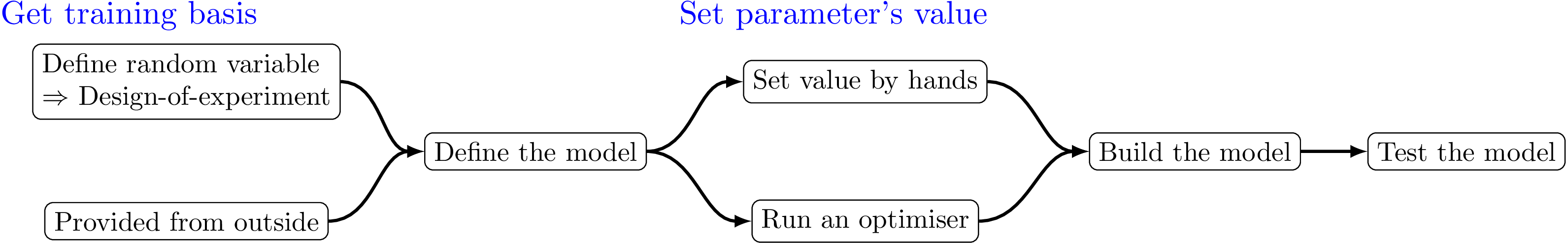
The kriging procedure in Uranie can be schematised in five steps, depicted in Figure V.4 and an example can be found in Section XIV.6.14. As for the polynomial chaos expansion discussed in Section V.3, the classes are mainly interfaces, here to the classes extracted from the gpLib library. Here is a brief description of the steps:

get a training site. Either produced by a design-of-experiments from a model definition, or taken from anywhere else, it is mandatory to get this basis (the larger, the better).
define the kriging options. This is heavily discussed in Section V.6.2, all the options discussed in the aforementioned section will be inputs of the TGPBuilder class that will be build the kriging model.
set the parameter's values. It can be set by hands, but it is highly recommended to proceed through an optimisation, to get the best possible parameters.
build the kriging method. This is done with a specific method of TGPBuilder which returns a TKriging object. This object is the one that would be saved (if requested) and used to perform the next step.
test the obtained kriging model. This is done by running the kriging model over a new basis (the test one) using a TLauncher2 object (which is the equivalent of a TLauncher but from the URANIE::Relauncher module). This module will be discussed later on in Chapter VIII. With this approach, a one-by-one estimation of the prediction is performed. To get the complete prediction with the new location covariance matrix (see [metho] for this theory behind this discussion) a different method has been introduced, see Section V.6.3.2.

Figure V.4. Schematic description of the kriging procedure as done within Uranie

V.6.2. Construction of a kriging model

V.6.2.1. Description of the main classes

The Uranie wrapper to the gpLib is based on 4 main classes:

TGPBuilder: allow to search for the optimal parameters of the correlation function and to build the kriging model;
TCorrelationFunction: parent class of the correlation functions used to model the spatial correlation of the observations;
TGPCostFunction: parent class of the criteria used to find the optimal parameters of the correlation function;
TKriging: used to predict new values (with confidence interval).

Most of the time, users will only need to use the TGPBuilder and TKriging classes.

V.6.2.2. Example: construction of a simple Kriging model

The example code below creates a prediction model of the type "simple kriging" (it can be found in Section XIV.6.9).

{
  // Load observations
  TDataServer *tdsObs = new TDataServer("tdsObs", "observations");
  tdsObs->fileDataRead("utf_4D_train.dat");
	
  // Construct the GPBuilder
  TGPBuilder *gpb = new TGPBuilder(tdsObs,            // observations data 
				   "x1:x2:x3:x4",     // list of input variables
				   "y",               // output variable
				   "matern3/2");      // name of the correlation function

  
  // Search for the optimal hyper-parameters
  gpb->findOptimalParameters("ML",            // optimisation criterion 
			     100,             // screening design size
			     "neldermead",    // optimisation algorithm
			     500);            // max. number of optimisation iterations
	
  // Construct the kriging model
  TKriging *krig = gpb->buildGP();
	
  // Display model information
  krig->printLog();

  }

In this script, after loading the observation data into a dataserver, we create a TGPBuilder object. To do so, one should provide the observations, the name of the attributes corresponding to the inputs, the name of the attribute corresponding to the output, and the name of the correlation function (here, it is a Matern 3/2 correlation function. The training (utf_4D_train.dat) and testing (utf_4D_test.dat) database can both be found in the document folder of the Uranie installation (${URANIESYS}/share/uranie/docUMENTS). Please refer to Table V.6 or [metho] for the list of available correlation functions).

The next step is to find the optimal parameters of the correlation function. To achieve this, we can use the TGPBuilder::findOptimalParameters function. It is a "helper function" where all the tedious work is done automatically. The drawback is that the user cannot modify some properties (parameters range, optimisation precision, etc.), or use some interesting features of Uranie (non-random sampling, evolutionary optimisation algorithms, distributed computing, etc.). Section V.6.4 gives some examples of how to search for optimal parameters without using the function findOptimalParameters.

The search for the optimal parameters requires the user to choose:

an optimisation criterion (in the example: the Maximum likelihood);
the size of the screening design-of-experiments;
an optimisation algorithm;
a maximum number of optimisation runs.

The search for optimal parameters will start by the search of a "good" starting point for the optimisation. This is done by evaluating the criterion on a LHS design-of-experiments of the input space. This "screening" procedure is optional and can be skipped by setting the design size to 0.

The optimisation procedure will start either at the "best" location found by the screening, or at a default location. The chosen optimisation algorithm is then used to search for an optimal solution. Depending on various conditions, convergence can be difficult to achieve. The number of optimisation runs is thus limited to 1000 by default, but can be increased or decreased by the user. The list of available optimisation criteria is available in Table V.4. The list of optimisation algorithms is available in Table V.5. You can also refer to the developer documentation.

When the search is finished, and if everything went well, we can create a kriging model using the function TGPBuilder::buildGP. This function returns the pointer to a TKriging object which can be used for the prediction of new points. The function TKriging::printLog shows some of the properties of the model, like the parameters of the correlation function and the leave one out performances (RMSE and Q2):

*******************************
** TKriging::printLog[]
*******************************
 Input Variables:      x1:x2:x3:x4
 Output Variable:      y
 Deterministic trend:  
 Correlation function: URANIE::Modeler::TMatern32CorrFunction
 Correlation length:   normalised   (not normalised)
                       1.6181e+00 (1.6172e+00 )
                       1.4372e+00 (1.4370e+00 )
                       1.5026e+00 (1.5009e+00 )
                       6.7884e+00 (6.7944e+00 )

 Variance of the gaussian process:      70.8755
 RMSE (by Leave One Out):               0.499108
 Q2:                                    0.849843
*******************************

Warning

Internally, the inputs are automatically normalised to the interval [0, 1]. As a consequence, the "normalised" correlation lengths correspond to distances in the normalised space, and the "not normalised" lengths correspond to distances in the original space.

V.6.2.3. Regularisation

Sometimes, the optimisation fails due to an ill-conditioned covariance matrix. The corresponding cost is set to an absurd value and this is signalled, at the end, by a warning message of the form (when XX estimations fail out of the total number TOT):

<WARNING> TGPBuilder::Screening procedure. The Cholesky decomposition has failed XX out of TOT times </WARNING>

It can then be useful to apply a regularisation parameter (mathematically similar to the "nugget effect" of geostatistics).

To apply the regularisation, we simply have to write:

gpb->setRegularisation(1e-6);

before calling findOptimalParameters. Typical values for the regularisation parameter lie between 1e-12 and 1e-6.

V.6.2.4. Deterministic trend and bayesian prior

Defining a deterministic trend is done at the construction of the TGPBuilder object. It can be generated automatically by using a keyword ("const" or "linear")

// Load observations
TDataServer *tdsObs = new TDataServer("tdsObs", "observations");
tdsObs->fileDataRead("utf_4D_train.dat");

// Construct the GPBuilder
TGPBuilder *gpb = new TGPBuilder(tdsObs,            // observations data 
"x1:x2:x3:x4",     // list of input variables
"y",               // output variable
"matern3/2",       // name of the correlation function
"linear");         // trend defined by a keyword

or manually by writing a formula where the terms are separated by colon character (":")

// Load observations
TDataServer *tdsObs = new TDataServer("tdsObs", "observations");
tdsObs->fileDataRead("utf_4D_train.dat");

// Construct the GPBuilder
TGPBuilder *gpb = new TGPBuilder(tdsObs,            // observations data 
"x1:x2:x3:x4",     // list of input variables
"y",               // output variable
"matern3/2",       // name of the correlation function
"1:x1:x2+x4^2");   // custom trend

When using the "const" keyword, the trend is a constant value. When using "linear", the trend is a linear combination of all the normalised input variables (plus a constant).

When using a formula, each sub-element must be either a constant or a combination of one or more inputs. It must also respect ROOT's formula syntax (cf. TFormula description for details).

Warning

Custom trend applies on "original space" variables, while automatic trend applies on "normalised space" variables.

This shows the impact of all deterministic trend cases implementation:

"": no trend given.
"const": There is an extra parameter to determine, as .
"linear": There are extra parameters to be determined, as .
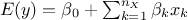"a:b:c": This is customised trend. The given string is split according to ":". There will be as many new parameters as there are entries and "a", "b", and "c" can be functions of various input variables. For instance with a line like , the trend would be

If we have an a priori knowledge on the mean and variance of the trend parameters, we can use it to perform a bayesian study, as in the example below (which can be found in Section XIV.6.11):

{
    // Load observations
   TDataServer *tdsObs = new TDataServer("tdsObs", "observations");
   tdsObs->fileDataRead("utf_4D_train.dat");
  
   // Construct the GPBuilder
   TGPBuilder *gpb = new TGPBuilder(tdsObs,            // observations data 
				    "x1:x2:x3:x4",     // list of input variables
				    "y",               // output variable
				    "matern3/2",       // name of the correlation function
				    "linear");         // trend defined by a keyword


   // Bayesian study
   Double_t meanPrior[5] = {0.0, 0.0, -1.0, 0.0, -0.1};
   Double_t covPrior[25] = {1e-4, 0.0 , 0.0 , 0.0 , 0.0 ,
			    0.0 , 1e-4, 0.0 , 0.0 , 0.0 ,
			    0.0 , 0.0 , 1e-4, 0.0 , 0.0 ,
			    0.0 , 0.0 , 0.0 , 1e-4, 0.0 ,
			    0.0 , 0.0 , 0.0 , 0.0 , 1e-4};
   gpb->setPriorData(meanPrior, covPrior);                                 
	
   // Search for the optimal hyper-parameters
   gpb->findOptimalParameters("ReML",          // optimisation criterion 
			      100,             // screening design size
			      "neldermead",    // optimisation algorithm
			      500);            // max. number of optimisation iterations
	
   // Construct the kriging model
   TKriging *krig = gpb->buildGP();
	
   // Display model information
   krig->printLog();

  }

Warning

Please note that we change the optimisation criterion from "ML" (Maximum likelihood) to "ReML" (Restricted Maximum likelihood) as the former cannot handle bayesian studies.

The information displayed by the TKriging::printLog function shows the values of the 5 trend parameters calculated by the bayesian study. The a priori variance of the parameters being very small, we can see that the trend parameters are very close to their a priori means.

*******************************
** TKriging::printLog[]
*******************************
 Input Variables:      x1:x2:x3:x4
 Output Variable:      y
 Deterministic trend:  linear
 Trend parameters (5): [3.06586494e-05; 1.64887174e-05; -9.99986787e-01; 1.51959859e-05; -9.99877606e-02 ]
 Correlation function: URANIE::Modeler::TMatern32CorrFunction
 Correlation length:   normalised   (not normalised)
                       2.1450e+00 (2.1438e+00 )
                       1.9092e+00 (1.9090e+00 )
                       2.0062e+00 (2.0040e+00 )
                       8.4315e+00 (8.4390e+00 )

 Variance of the gaussian process:      155.533
 RMSE (by Leave One Out):               0.495448
 Q2:                                    0.852037
*******************************

Tip

If you want to deactivate the bayesian mode after setting the prior data, call gpb->setUsePrior(kFALSE) before searching for the optimal parameters. You can reactivate the bayesian mode later by calling gpb->setUsePrior(kTRUE).

V.6.2.5. Measurement error

If we want to take a measurement error into account when looking for the optimal hyper-parameters, we can do so by calling the function:

gpb->setHasMeasurementError(kTRUE);

The measurement error is supposed to follow a normal law of mean 0. If the variance vMes is unknown, a new parameter alpha = vMes/vGP (where vGP is the variance of the gaussian process) will be added to the list of hyper-parameters to optimise.

If we know the variance of the measurement error to be a constant, it must be set using the function

Double_t vMes = 0.0025;
gpb->setMeasurementErrorVariance(vMes);

We may even know the covariance matrix of a complex measurement error. In such case, it must be set using the function

Double_t covMes[25] = {25*1e-4, 0.0 ,    0.0 , 0.0 ,    0.0 ,
0.0 , 25*1e-4, 0.0 , 0.0 ,    0.0 ,
0.0 , 0.0 , 25*1e-4, 0.0 ,    0.0 ,
0.0 , 0.0 ,    0.0 , 25*1e-4, 0.0 ,
0.0 , 0.0 ,    0.0 , 0.0 , 25*1e-4};
gpb->setMeasurementErrorCovMatrix(covMes);

In both cases, the variance of the gaussian process, which is otherwise determined analytically from the other hyper-parameters, becomes one of the hyper-parameters to optimise.

V.6.2.6. Optimisation options

The optimisation phase of the search for optimal parameters depends on the choice of a criterion and an optimisation algorithm. In the tables below, we present a quick description of the available options.

Table V.4. Optimisation criteria

Criteria	keyword	no trend	trend	bayesian	description
Maximum likelihood	ML	yes	yes	no	Look for the hyper-parameters which maximise the density of the gaussian vector of the observation outputs. It cannot be used for bayesian studies.
Restricted Maximum likelihood	ReML	no	yes	yes	Same as ML, but adapted to allow bayesian studies. It cannot be used without a trend.
Leave One Out	Loo	yes	yes	yes	Thanks to the linear nature of the kriging model, the Leave One Out error has an analytic formulation. It can be used as a quality criterion.

Table V.5. Optimisation algorithm

Algorithm	keyword	Use gradient	description
Nelder-Mead Simplex	NelderMead	no	This is an implementation of the "simplex" algorithm, simple and quite efficient in most cases. However, it does not always converge to a local minimum
Subplex	Subplexe^[a]	no	Another version of the simplex supposed to be more robust and efficient than Nelder-Mead
Constrained Optimisation By Linear Approximations	Cobyla	no	Construct successive linear approximations of the cost function (using a simplex) and optimise them.
Bound Optimisation BY Quadratic Approximation	Bobyqa	no	Construct quadratic approximations of the cost function and optimise them. May perform poorly on cost function that are not twice-differentiable !
Principal Axis	Praxis	no	Use the "principal axis" method to converge to a solution without estimating a gradient. May be slow to converge.
Low-storage BFGS	BFGS	yes	An improved implementation of the BFGS algorithm which reduces memory consumption and convergence time.
Preconditioned truncated Newton	Newton	yes	An implementation of the Newton algorithm which reduces memory consumption and convergence time.
Method of Moving Asymptotic	MMA	yes	Construct local approximation of the cost function based on the gradient, the constraints and a quadratic "penalty" term. The approximation obtained is "easy" to optimise. This algorithm is guaranteed to converge to a local minimum whatever the starting point.
Sequential Least-Squares Quadratic Programming	SLSQP	yes	The algorithm optimises successive second-order approximations of the cost function (via BFGS updates), with first-order (linear) approximations of the constraints. As it uses "true" BFGS, this algorithm becomes slow for large numbers of parameters
Shifted limited-memory variable-metric	VariableMetric	yes	This algorithm is adapted to large scale optimisation problems.
^[a]the additional "e" is to respect the original author's wish that only his implementation of the algorithm be named "Subplex".

For more details about the algorithms, please consult the NLopt website ( http://ab-initio.mit.edu/wiki/index.php/NLopt_Algorithms).

V.6.2.7. Choice of the initial point of the optimisation

In the examples presented so far, the initial point of the optimisation procedure was either a default location or determined via a random sampling of the input space. If a specific location is needed, it can be set as shown below (which can be found in Section XIV.6.10):

{
 // Load observations
 TDataServer *tdsObs = new TDataServer("tdsObs", "observations");
 tdsObs->fileDataRead("utf_4D_train.dat");
 
 // Construct the GPBuilder
 TGPBuilder *gpb = new TGPBuilder(tdsObs, "x1:x2:x3:x4", "y", "matern3/2");
 
 // Set the correlation function parameters
 Double_t params[4] = {1.0, 0.25, 0.01, 0.3};
 gpb->getCorrFunction()->setParameters(params);

 // Find the optimal parameters
 gpb->findOptimalParameters("ML",         // optimisation criterion 
                            0,            // screening size MUST be equal to 0 
			    "neldermead", // optimisation algorithm
			    500,          // max. number of optimisation iterations
			    kFALSE);      // we don't reset the parameters of the GP builder
      
  // Create the kriging model
  TKriging *krig = gpb->buildGP();
      
  // Display model information
  krig->printLog();                

  }

In this case, only the initial correlation lengths need to be set, so we simply retrieve the pointer to the correlation function object and use the setParameters function. Then, we call findoptimalParameters with two particularities:

the screening size must be set to 0, otherwise the initial point will be defined as the best location of a random sampling;
the last parameter of the function, called "reset", must be set to kFALSE. This insures that the current values of the hyper-parameters are not reset to their default values.

Warning

When setting the correlation lengths manually, remember that the values you provide are considered normalised.

The resulting model is printed as follow:

*******************************
** TKriging::printLog[]
*******************************
 Input Variables:      x1:x2:x3:x4
 Output Variable:      y
 Deterministic trend:  
 Correlation function: URANIE::Modeler::TMatern32CorrFunction
 Correlation length:   normalised   (not normalised)
                       1.6182e+00 (1.6173e+00 )
                       1.4373e+00 (1.4371e+00 )
                       1.5027e+00 (1.5011e+00 )
                       6.7895e+00 (6.7955e+00 )

 Variance of the gaussian process:      70.8914
 RMSE (by Leave One Out):               0.49911
 Q2:                                    0.849842
*******************************

V.6.2.8. Observations update

One situation where it might be interesting to continue an optimisation procedure from the last optimal solution found is when the observation dataset is updated "on the fly". A typical use-case is the iterative construction of a design-of-experiments.

If the contents of the dataserver of the observations are modified, we must update the internal matrices of the TGPBuilder, but without modifying the hyper-parameters we have found so far. The function TGPBuilder::updateObservations does exactly that:

{
  // Load observations
  TDataServer *tdsObs = new TDataServer("tdsObs","");
  tdsObs->fileDataRead("utf_4D_train.dat");

  // Construct the GPBuilder        
  TGPBuilder *gpb = new TGPBuilder(tdsObs, "x1:x2:x3:x4", "y", "matern3/2");

  // Search for the optimal hyper-parameters
  gpb->findOptimalParameters("ML", 100, "neldermead", 500);
  
  // Create a new observation
  Double_t newObs[5] = {7.547605e-01, 8.763968e-01, 1.255390e-01, 6.370434e-01, 1.189220e+00};
      
  // Add the new observation to tdsObs
  Double_t newLine[6];
  newLine[0] = tdsObs->getNPatterns()+1; // Index of the new observation
  newLine[1] = newObs[0];
  newLine[2] = newObs[1];
  newLine[3] = newObs[2];
  newLine[4] = newObs[3];
  newLine[5] = newObs[4];
  
  tdsObs->getTuple()->Fill(newLine);

  // Update the GP Builder
  gpb->updateObservations();
  
  // Search for the new optimal hyper-parameters, starting from their current values 
  gpb->findOptimalParameters("ML", 0, "bobyqa", 500, kFALSE);

  // Create the model
  TKriging *krig = gpb->buildGP();
      
  // Display model information
  krig->printLog();                                
  
  }

The resulting model is printed as follow:

*******************************
** TKriging::printLog[]
*******************************
 Input Variables:      x1:x2:x3:x4
 Output Variable:      y
 Deterministic trend:  
 Correlation function: URANIE::Modeler::TMatern32CorrFunction
 Correlation length:   normalised   (not normalised)
                       1.6272e+00 (1.6263e+00 )
                       1.4443e+00 (1.4441e+00 )
                       1.5095e+00 (1.5078e+00 )
                       6.8387e+00 (6.8447e+00 )

 Variance of the gaussian process:      71.8595
 RMSE (by Leave One Out):               0.498229
 Q2:                                    0.85008
*******************************

V.6.3. Usage of a Kriging model

V.6.3.1. Prediction of a new data set, one-by-one approach

In the following example, we use a newly constructed kriging model to estimate the output of a new dataset (the code can be found in Section XIV.6.12):

{
  // Load observations
  TDataServer *tdsObs = new TDataServer("tdsObs", "observations");
  tdsObs->fileDataRead("utf_4D_train.dat");
      
  // Construct the GPBuilder
  TGPBuilder *gpb = new TGPBuilder(tdsObs,            // observations data 
				   "x1:x2:x3:x4",     // list of input variables
				   "y",               // output variable
				   "matern3/2");       // name of the correlation function

                    
  // Search for the optimal hyper-parameters
  gpb->findOptimalParameters("ML",            // optimisation criterion 
			     100,             // screening design size
			     "neldermead",    // optimisation algorithm
			     500);            // max. number of optimisation iterations
      
  // Construct the kriging model
  TKriging *krig = gpb->buildGP();
      
  // Display model information
  krig->printLog();
      
  // Load the data to estimate
  TDataServer *tdsEstim = new TDataServer("tdsEstim", "estimations");
  tdsEstim->fileDataRead("utf_4D_test.dat");
      
  // Construction of the launcher
  TLauncher2 *lanceur = new TLauncher2(tdsEstim,          // data to estimate
				       krig,              // model used for the estimation
				       "x1:x2:x3:x4",     // list of the input variables
				       "yEstim:vEstim");  // name given to the model's outputs 
      
  // Launch the estimations
  lanceur->solverLoop();
      
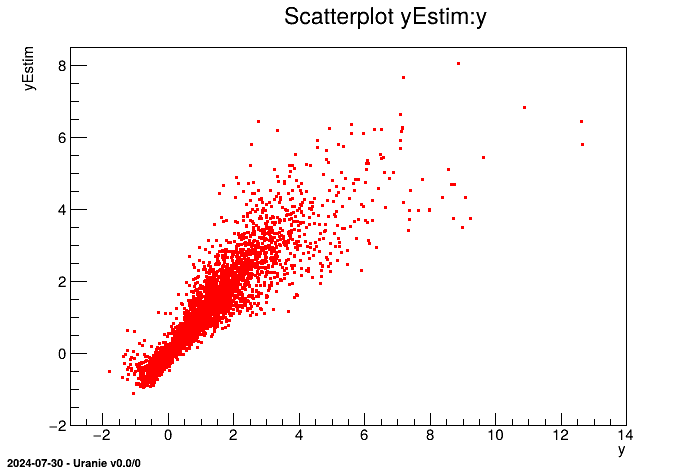
  // Display some results
  tdsEstim->draw("yEstim:y");

  }

The part where the kriging model is constructed is identical to Section V.6.2.2.

After printing the model information, the new data are loaded into a dataserver. The TKriging class is a children of TSimpleEval and can thus be used by a TMaster (cf. Chapter VIII). Here, we create a TLauncher2 object. It receives the data to estimate, the model to apply, the names of the input variables, and the names of the output variable. The latter is added to the dataserver and receive the responses of the model when the function solverLoop is called.

Warning

Using the prototype shown above (and recall here) to construct TLauncher2 instance is perfectly fine as long as one does not want to use constant or temporary attributes. If you don't know what's discussed here, we strongly invite you to have a look here Section VIII.5.1.

TLauncher2(TDataServer *tds, TStandardEval *fun, const char *in, const char *out);

Even though one can define at once the input and output attributes (that should be in the input TDataServer) but there is no way to state that one input attribute is constant to set its value later-on just before the solverLoop call. In order to do that, one should stick to the "classical" Relauncher architecture:

add input attributes to the evaluator using the addInput and / or setInputs methods;
add output attributes to the evaluator using the addOutput and / or setOutputs methods;

create the TLauncher2 instance with this prototype

TLauncher2(TDataServer *tds, TStandardEval *fun);

For each point of the data set, we now have an estimation of the output ("yEstim") and a variance of this estimation ("vEstim"). We can access these values via the dataserver's visualisation or computation tools.

Figure V.5. Estimation using a simple Kriging model

V.6.3.2. Prediction of a new data set, global approach

In the following example, we use a newly constructed kriging model to estimate the output of a new dataset, but unlike the previous case (see Section V.6.3.1) the prediction is done at once, taking into account the covariance of the new locations input to produce the prediction covariance matrix. The code can also be bound in Section XIV.6.13.

{
  // Load observations
  TDataServer *tdsObs = new TDataServer("tdsObs", "observations");
  tdsObs->fileDataRead("utf_4D_train.dat");
      
  // Construct the GPBuilder
  TGPBuilder *gpb = new TGPBuilder(tdsObs,            // observations data 
				   "x1:x2:x3:x4",     // list of input variables
				   "y",               // output variable
				   "matern1/2");       // name of the correlation function

                    
  // Search for the optimal hyper-parameters
  gpb->findOptimalParameters("ML",            // optimisation criterion 
			     100,             // screening design size
			     "neldermead",    // optimisation algorithm
			     500);            // max. number of optimisation iterations
      
  // Construct the kriging model
  TKriging *krig = gpb->buildGP();
      
  // Display model information
  krig->printLog();
      
  // Load the data to estimate
  TDataServer *tdsEstim = new TDataServer("tdsEstim", "estimations");
  tdsEstim->fileDataRead("utf_4D_test.dat");

  // Reducing the database to 1000 first event (prediction cov matrix of a million value !)
  int nST=1000;
  tdsEstim->exportData("utf_4D_test_red.dat","",Form("tdsEstim__n__iter__<=%d",nST));
  tdsEstim->fileDataRead("utf_4D_test_red.dat",false,true); // Reload reduce sample    

 krig->estimateWithCov(tdsEstim, // data to estimate
                        "x1:x2:x3:x4",// list of the input variables
                        "yEstim:vEstim", // name given to the model's outputs
                        "y", //name of the true reference if validation database
                        ""); //options

  TCanvas *c2=NULL;
  // Residuals plots if true information provided
  if( tdsEstim->isAttribute("_Residuals_") ) 
  {
      c2 = new TCanvas("c2","c2",1200,800);
      c2->Divide(2,1);
      c2->cd(1);
      // Usual residual considering uncorrated input points
      tdsEstim->Draw("_Residuals_"); 
      c2->cd(2);
      // Corrected residuals, with prediction covariance matrix
      tdsEstim->Draw("_uncorrResiduals_"); 
  }

  // Retrieve all the prediction covariance coefficient
  tdsEstim->getTuple()->SetEstimate( nST * nST ); //allocate the correct size
  // Get a pointer to all values
  tdsEstim->getTuple()->Draw("_CovarianceMatrix_","","goff");
  double *cov=tdsEstim->getTuple()->GetV1();

  //Put these in a matrix nicely created
  TMatrixD Cov(nST,nST);
  Cov.Use(0,nST-1,0,nST-1,cov);

  //Print it if size is reasonnable
  if(nST<10)
      Cov.Print();

  }

The part where the kriging model is constructed is identical to Section V.6.2.2.

After printing the model information, the new data are loaded into a dataserver. Unlike the previous case (see Section V.6.3.1), the validation database is reduced to a fifth of its original size, as the global approach will have to compute the input covariance matrix but also, from it, the prediction covariance matrix, both of which have, just for the reduced case, a million coefficients. The method to do this is called estimateWithCov and it can take 5 parameters:

a pointer to the dataserver;
the list of inputs to be used;
the name of the outputs. Only two are allowed and compulsory: the predicion and its conditional variance;
the name of the true value of the model (optional). Usable only with validation / test database;
and the options.

For each point of the data set, we now have an estimation of the output ("yEstim") and a variance of this estimation ("vEstim"). This method also produce few more attributes:

"_CovarianceMatrix_": this is a strange way to store the final prediction covariance matrix. It is a new vector attribute whose size is constant throughout the dataserver and it is the size of the sample. For every entry it corresponds to the row of the covariance matrix and the recommended way to extract it is the way shown above, i.e.


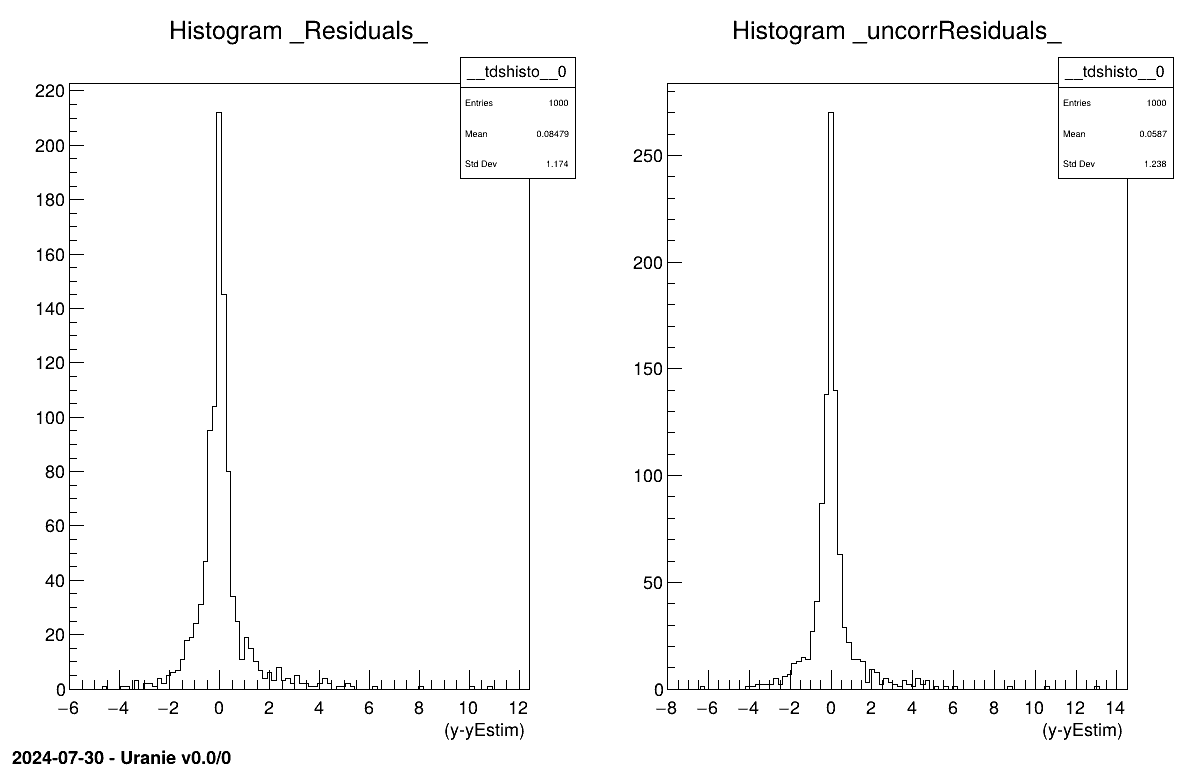
// Retrieve all the prediction covariance coefficient
tdsEstim->getTuple()->SetEstimate( nST * nST ); //allocate the correct size
// Get a pointer to all values
tdsEstim->getTuple()->Draw("_CovarianceMatrix_","","goff");
double *cov=tdsEstim->getTuple()->GetV1(); // The data itself
  
//Put these in a matrix nicely created (high level object to deal with)
TMatrixD Cov(nST,nST);
Cov.Use(0,nST-1,0,nST-1,cov);

"_Residuals_" and "_uncorrResiduals_": available only if the true value of the model is provided along (as fourth parameter of the function prototype). It is basically the following ratio for all locations in the tested database P:
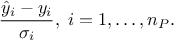
It is depicted in our case in Figure V.6.

Figure V.6. Residual distribution using a validation database with and without prediction covariance correction.

V.6.3.3. Saving and loading a model

It is not currently possible to export a kriging model as a standalone C or fortran function. There are various reasons for this. The main one is that saving a kriging model means saving several matrices which can be huge when the number of observations and/or the number of input variables is large. It is thus impractical to save them in a text format as is usually done for the other algorithms of URANIE::Modeler.

The alternative is to export the information needed to build the TKriging object with a TGPBuilder. This is done by the function exportGPData:

gpb->findOptimalParameters("ML",100,"neldermead",500);

// export optimal parameters to a file
gpb->exportGPData("modelData.dat");

The file created ("modelData.dat") is a standard "Salome table" file, with a special #TITLE line in its header:

#NAME: tdsKriging
#TITLE: URANIE::Modeler::TMatern32CorrFunction: [1.61744349e+00 1.43718257e+00 1.50122179e+00 6.79556828e+00]; variance: 7.09060005e+01; 
#DATE: Wed Aug  6 10:24:36 2014
#COLUMN_NAMES: x1| x2| x3| x4| y| tdsKriging__n__iter__

2.186488000e-01 1.534173000e-01 6.196718000e-01 3.452344000e-01 1.235132000e+00 1
9.467816000e-02 3.830201000e-01 5.978722000e-03 7.689013000e-01 2.527613000e+00 2
4.716125000e-01 1.566920000e-01 8.623332000e-01 9.878017000e-01 -6.464496000e-01 3
1.346335000e-01 7.979628000e-02 5.091562000e-01 7.396531000e-01 2.461238000e+00 4
6.238671000e-01 2.995599000e-01 2.385627000e-01 9.548934000e-01 -3.266630000e-03 5
...

The #TITLE line contains the class name of the correlation function, its parameters, the variance of the gaussian process, and any other parameter required to construct the kriging model. The rest of the file contains the observation inputs and output.

Warning

Do not modify the content of the file unless you know exactly what you are doing. It may produce a model which has nothing to do with the original one, or the file may not be readable at all.

The script below presents how to reconstruct the model from the saved file:

{  
 // Load the model data file into a data server
 TDataServer *tdsModelData = new TDataServer(); // VERY IMPORTANT: do not give any name or title to this tds !
 tdsModelData->fileDataRead("modelData.dat");
      
 // Create a GP builder based on this data server
 TGPBuilder *gpb = new TGPBuilder(tdsModelData);

 // Create the kriging model
 TKriging *krig = gpb->buildGP();

 // Display model information
 krig->printLog();        

  }

The constructor of the TGPBuilder object takes only the dataserver with the model data. It reads the #TITLE line and extracts the information. It is thus not necessary to call findOptimalParameters. The function buildGP can be used immediately to create the model. This macro is finished by printing the resulting model:

*******************************
** TKriging::printLog[]
*******************************
 Input Variables:      x1:x2:x3:x4
 Output Variable:      y
 Deterministic trend:  
 Correlation function: URANIE::Modeler::TMatern32CorrFunction
 Correlation length:   normalised   (not normalised)
                       9.7238e-01 (9.7183e-01 )
                       8.5615e-01 (8.5606e-01 )
                       9.4116e-01 (9.4013e-01 )
                       4.3909e+00 (4.3948e+00 )

 Variance of the gaussian process:      18.1787
 RMSE (by Leave One Out):               0.510406
 Q2:                                    0.842968
*******************************

V.6.4. Advanced usage

The function TGPBuilder::findOptimalParameters greatly simplifies the process of finding good parameters for the correlation function. However, in some cases, it might be interesting to perform this procedure differently. In the following sections, we go "inside the engine" to allow advanced users to go beyond findOptimalParameters if they want to.

V.6.4.1. The correlation function

A TGPBuilder object contains a TCorrelationFunction object which will compute the correlation between the observation points. A clone of this correlation function object is stored in the TKriging object, where it will estimate the correlation between the observations and a new point.

It is possible to set the correlation function object manually, either at construction, or later using TGPBuilder::setCorrFunction. Whether the user creates a new object or simply passes a keyword to the TGPBuilder, a new correlation function object will be created inside the TGPBuilder and destroyed with it.

The example below illustrates the construction of a TGPBuilder by passing a correlation function object:

...      
// Definition of the initial correlation lengths
Double_t corrLengths[4] = {1.0, 0.25, 0.01, 0.3};

// Construction of the correlation function
TMatern32CorrFunction *corrFunc = new TMatern32CorrFunction(4, corrLengths);

// Construction of the GP builder
TGPBuilder *gpb = new TGPBuilder(tdsObs, "x1:x2:x3:x4", "y", corrFunc);

// The correlation function object is no longer needed. We can destroy it
delete corrFunc;
...

The table below presents the list of correlation functions currently available in Uranie:

Table V.6. Correlation functions

Class Name	keyword	number of parameters^[a]	order of the parameters in the parameters array ^[b]
TExponentialCorrFunction	exponential	2*d	[ p1, p2, ..., pd, l1, l2,..., ld ]
TGaussianCorrFunction	gauss	d	[ l1, l2,..., ld ]
TIsotropicGaussianCorrFunction	isogauss	1	[ l ]
TMaternICorrFunction	maternI	2*d	[ v1, v2, ..., vd, l1, l2,..., ld ]
TMaternIICorrFunction	maternII	d+1	[ v, l1, l2,..., ld ]
TMaternIIICorrFunction	maternIII	d+1	[ v, l1, l2,..., ld ]
TMatern12CorrFunction	matern1/2	d	[ l1, l2,..., ld ]
TMatern32CorrFunction	matern3/2	d	[ l1, l2,..., ld ]
TMatern52CorrFunction	matern5/2	d	[ l1, l2,..., ld ]
TMatern72CorrFunction	matern7/2	d	[ l1, l2,..., ld ]
^[a]d is the number of dimensions of the input space ^[b]p is the power of the exponential; v is the regularisation parameter of the Matèrn function; l is the correlation length.

For a more complete description of the available correlation functions (at least a more mathematical one) please report to [metho].

V.6.4.2. The cost function

As mentioned before, Uranie provides three criteria (or cost functions) to select "good" hyper-parameters for the kriging model. If needed, the user can create his own TGPCostFunction object and apply his own searching method to find the optimal hyper-parameters.

The TGPCostFunction classes inherit from TSimpleEval and can thus be used by a TMaster (cf. Chapter VIII). Complete examples of how to use a cost function object are given in the next sections.

V.6.4.3. Example: parameters searched by LHS

The example below illustrate the "manual" search for optimal hyper-parameters through a screening of the parameters space.

{
 using namespace URANIE::DataServer; // TDataServer, TLogUniformDistribution
 using namespace URANIE::Modeler;    // TGPBuilder, TGPMLCostFunction, TKriging 
 using namespace URANIE::Sampler;    // TBasicSampling
 using namespace URANIE::Relauncher; // TLauncher2
      
 // Load observations
 TDataServer *tdsObs = new TDataServer("tdsObs","");
 tdsObs->fileDataRead("utf_4D_train.dat");

 // Construct the GPBuilder        
 TGPBuilder *gpb = new TGPBuilder(tdsObs, "x1:x2:x3:x4", "y", "matern3/2");

 // construction of the cost function
 TGPMLCostFunction *cost = new TGPMLCostFunction(gpb);
      
 //----------------------------------//
 // Construction of the LHS sampling //
 //----------------------------------//
 // construction of the attributes
 TLogUniformDistribution *cl1 = new TLogUniformDistribution("cl1", 1e-6, 10.0);
 TLogUniformDistribution *cl2 = new TLogUniformDistribution("cl2", 1e-6, 10.0);
 TLogUniformDistribution *cl3 = new TLogUniformDistribution("cl3", 1e-6, 10.0);
 TLogUniformDistribution *cl4 = new TLogUniformDistribution("cl4", 1e-6, 10.0);
 
 // Construction of the data server containing the exploration 
 // of the correlation lengths' space
 TDataServer *tdsParam = new TDataServer("tdsParam", "");
 tdsParam->addAttribute(cl1);
 tdsParam->addAttribute(cl2);
 tdsParam->addAttribute(cl3);
 tdsParam->addAttribute(cl4);
 
 // Construction of the sampler and generation of the data
 Int_t screeningSize = 1000;
 TBasicSampling *s = new TBasicSampling(tdsParam, "lhs", screeningSize);
 s->generateSample();
 
 // Evaluate the cost function on the sampling
 TLauncher2 *l = new TLauncher2(tdsParam,cost,"cl1:cl2:cl3:cl4","cost:varGP");
 l->solverLoop();
 
 //-----------------------------------------------------------//
 // Search for the minimum value of the cost and retrieve the //
 // corresponding correlation lengths                         //
 //-----------------------------------------------------------//
 // Retrieve the cost values
 Double_t *costValues = tdsParam->getTuple()->getBranchData("cost");
 
 // find the index of the minimum cost
 Int_t minIndex = TMath::LocMin(screeningSize, costValues);
 Double_t optimalCost = costValues[minIndex];
 
 // retrieve the values of the optimal correlation lengths 
 Double_t optimalParams[4];
 optimalParams[0] = tdsParam->getValue("cl1", minIndex);
 optimalParams[1] = tdsParam->getValue("cl2", minIndex);
 optimalParams[2] = tdsParam->getValue("cl3", minIndex);
 optimalParams[3] = tdsParam->getValue("cl4", minIndex);
 
 // retrieve the value of the GP variance
 Double_t optimalVar = tdsParam->getValue("varGP", minIndex);  
 
 //-----------------------------------------------------------//
 // Update the GP Builder with the newly found parameters and //
 // create the model                                          //
 //-----------------------------------------------------------//
 // set the parameters of the correlation function
 gpb->getCorrFunction()->setParameters(optimalParams);
 
 // set the GP variance
 gpb->setVariance(optimalVar);
 
 // Create the model
 TKriging *krig = gpb->buildGP();
 
 // Display model information
 krig->printLog();    
      
  }

The first step of the procedure is similar to what we have seen so far: we are loading the observations into a data server and create a TGPBuilder. The change occurs when we create a TGPMLCostFunction object. It will allow us to evaluate the likelihood of the gaussian process for a given set of hyper-parameters. For this, it needs an access to the observations, the correlation function, etc. This is done by giving it a pointer to the TGPBuilder object.

The next step is to create the dataset which will allow us to explore the parameter space. In this example, we only care about the correlation lengths along each of the 4 input variables. We create a TLogUniformDistribution object for each of them in order to have a good screening resolution on small correlation lengths. Then, we create the dataserver that will hold the dataset, add the attributes to it, create a sampler object and generate the data (cf. Chapter III for details).

When the dataset is ready, we need to evaluate the cost function on it. An easy way to do it is to create a TLauncher2 object, and give it the dataset, the cost function object, the input names, and the output names. When the function solverLoop is called, the entries of the dataset are sent to the cost function, and the results of the latter are stored in the dataserver.

The next operation is the retrieval of the optimal parameters. We need to identify the point with the minimal cost, and extract the values of the corresponding correlation lengths and GP variance. When done, we need to manually update the TGPBuilder. First, we set the new parameters of the correlation function by retrieving the correlation function pointer (using TGPBuilder::getCorrFunction), and by calling TCorrelationFunction::setParameters. Then, we set the variance of the gaussian process by calling TGPBuilder::setVariance.

At this stage, the TGPBuilder object is ready to create a kriging model with the new hyper-parameters found. This is what we do by calling buildGP.

This example is a simplified version of what is done inside findOptimalParameters. But here, we can decide to distribute the computations, use another screening procedure, etc. We can even use another cost function !

The resulting model is printed as follow:

*******************************
** TKriging::printLog[]
*******************************
 Input Variables:      x1:x2:x3:x4
 Output Variable:      y
 Deterministic trend:  
 Correlation function: URANIE::Modeler::TMatern32CorrFunction
 Correlation length:   normalised   (not normalised)
                       4.4685e-01 (4.4660e-01 )
                       2.3956e-01 (2.3953e-01 )
                       2.9826e-01 (2.9794e-01 )
                       1.6450e+00 (1.6464e+00 )

 Variance of the gaussian process:      1.89625
 RMSE (by Leave One Out):               0.578768
 Q2:                                    0.798086
*******************************

V.6.4.4. Example: parameters search by direct optimisation

The example below illustrate the "manual" search for optimal hyper-parameters through a direct optimisation.

{
  using namespace URANIE::DataServer; // TDataServer, TLogUniformDistribution
  using namespace URANIE::Modeler;    // TGPBuilder, TGPMLCostFunction, TKriging 
  using namespace URANIE::Reoptimizer;// TNlopt, TNloptNelderMead
  
  // Load observations
  TDataServer *tdsObs = new TDataServer("tdsObs","");
  tdsObs->fileDataRead("utf_4D_train.dat");
  
  // Construction of the GPBuilder        
  TGPBuilder *gpb = new TGPBuilder(tdsObs, "x1:x2:x3:x4", "y", "matern3/2");
  
  // Construction of the cost function
  TGPMLCostFunction *costFunc = new TGPMLCostFunction(gpb);
  
  //--------------------------------------------//
  // Construction of the parameters to optimise //
  //--------------------------------------------//
  // construction of the input attributes 
  TAttribute *cl1 = new TAttribute("cl1", 1e-6, 10.0);
  TAttribute *cl2 = new TAttribute("cl2", 1e-6, 10.0);
  TAttribute *cl3 = new TAttribute("cl3", 1e-6, 10.0);
  TAttribute *cl4 = new TAttribute("cl4", 1e-6, 10.0);
  // construction of the output attributes
  TAttribute *cost  = new TAttribute("cost");
  TAttribute *varGP = new TAttribute("varGP");
  
  // Construction of the data server containing the parameters to optimise
  TDataServer *tdsParam = new TDataServer("tdsParam", "");
  tdsParam->addAttribute(cl1);
  tdsParam->addAttribute(cl2);
  tdsParam->addAttribute(cl3);
  tdsParam->addAttribute(cl4);
  
  // Add the parameters to optimise to the cost function
  costFunc->setInputs(4, cl1, cl2, cl3, cl4);
  costFunc->setOutputs(2, cost, varGP);
  
  //-------------------------------//
  // Construction of the optimiser //
  //-------------------------------//       
  // Choice of an optimisation algorithm
  TNloptNelderMead *solver = new TNloptNelderMead();
  
  // Construction of the optimizer, which receives the data server storing 
  // the optimal result, the criterion and the optimisation algorithm.
  TNlopt *opt = new TNlopt(tdsParam, costFunc, solver);
  
  // Optimisation options
  opt->addObjective(cost); // criterion to minimise    
  vector<double> start{1e-2, 1e-2, 1e-2, 1e-2};
  opt->setStartingPoint(start.size(),&start[0]); // starting point for the optimisation
  opt->setMaximumEval(1000); // maximum number of evaluation calls 
  opt->setTolerance(1e-12); // convergence criterion
  
  // Launch the optimisation procedure
  opt->solverLoop();
  
  //-----------------------------------------------------------//
  // Update the GP Builder with the newly found parameters and //
  // create the model                                          //
  //-----------------------------------------------------------//
  // Retrieve the optimal parameters. In this case, the data server contains only
  // one set of parameters, thus we don't have to search for the minimal cost.
  Double_t optimalParams[4];
  optimalParams[0] = tdsParam->getValue("cl1",0);
  optimalParams[1] = tdsParam->getValue("cl2",0);
  optimalParams[2] = tdsParam->getValue("cl3",0);
  optimalParams[3] = tdsParam->getValue("cl4",0);
  // set the parameters of the correlation function
  gpb->getCorrFunction()->setParameters(optimalParams);    
  
  // Retrieve the computed variance
  Double_t optimalVar = tdsParam->getValue("varGP",0);
  // Set the new variance of the GP
  gpb->setVariance(optimalVar);
  
  // Create the model
  TKriging *krig = gpb->buildGP();
  
  // Display model information
  krig->printLog();    

  }

The beginning of the script is the same as in the previous example (see Section V.6.4.3). The first difference concerns the construction of the attributes representing the parameters to optimise. Here, we do not need to define a distribution for the variables: we just need boundaries. This is the reason why all the input attributes are TAttribute objects, with a minimum and maximum value. The output attributes have no predefined boundaries.

After defining the input and output attributes, we need to create a dataserver to store the results of the optimisation. We provide it only with the input attributes. The output attributes will be automatically added during the optimisation procedure. We also need to tell the cost function which attributes represent the parameters to optimise, and which attributes represents the outputs of the cost function.

The next step is the construction of the optimiser. As explained in Chapter IX, an optimiser needs three objects to perform an optimisation procedure: a dataserver to store the results, a cost function to evaluate the criterion (or the criteria, for multi-objectives optimisation), and an optimisation algorithm to propose a new set of input parameters. The two former objects are already created. In our example, the latter is a TNloptNelderMead object.

Once constructed, the optimiser object must receive some additional information before starting the procedure. The first one are the output attributes of the cost function corresponding which correspond to the criteria. In this example, we have only one criterion: the attribute "cost" which refers to the negative log-likelihood of the gaussian process. The second mandatory information is the starting point of the optimisation. More than one starting point can be provided. As many optimal set of parameters will be stored in the dataserver. Finally, non mandatory options can be set, like the maximum number of evaluations of the cost function, or the tolerance criterion used to consider that the optimisation has converged to a solution. When everything is set, we can launch the optimisation procedure by calling the solverLoop function.

Retrieving the optimal parameters is easier in this case than in the LHS: only the optimal solutions for each starting point are stored in the dataserver ! As we have only one starting point in this example, we have only one solution to extract and provide to the TGPBuilder. Once done, we can create our kriging model as we did before.

The resulting model is printed as follow:

*******************************
** TKriging::printLog[]
*******************************
 Input Variables:      x1:x2:x3:x4
 Output Variable:      y
 Deterministic trend:  
 Correlation function: URANIE::Modeler::TMatern32CorrFunction
 Correlation length:   normalised   (not normalised)
                       1.6180e+00 (1.6171e+00 )
                       1.4371e+00 (1.4369e+00 )
                       1.5025e+00 (1.5009e+00 )
                       6.7885e+00 (6.7944e+00 )

 Variance of the gaussian process:      70.8649
 RMSE (by Leave One Out):               0.49911
 Q2:                                    0.849841
*******************************


V.5. The artificial neural network		Chapter VI. The Sensitivity module