

Documentation
/ Manuel utilisateur en C++
: 
| VI.7. The Johnson relative weight | ||
|---|---|---|
 | Chapter VI. The Sensitivity module |  |
This section introduces indices whose purpose is mainly to obtain good estimators of the Shapley's values defined in [metho]. The underlying assumption is to state that the model can be considered linear so that the results can be considered as proper estimation of the Shapley indices (with or without correlation between the input variables).
In Uranie, computing sensitivity indices with Johnson's relative weights method is dealt with the eponymous class
TJohnsonRW which inherits from the TSensitivity class.
This class handles all the steps to compute the indices depending on provided informations:
- one can only provide a correlation matrix without data. The indices would be estimated as such.
- one can provide a sample containing input and outputs variables. From there the class will compute the correlation matrix and estimate the indeces from them.
- If one provides either a code, a function, or a runner (see Section VIII.4) then, the class can
- generate the deterministic sample if no data are found;
- run the code, the analytic function or the evaluator if the output is not provided as well;
- computing the indices.
The example script below uses the TJohnsonRW class to compute and display the relative
weights:
{
gROOT->LoadMacro("UserFunctions.C");
// Define the DataServer
TDataServer *tds = new TDataServer("tdsflowrate", "DataBase flowrate");
tds->addAttribute( new TUniformDistribution("rw", 0.05, 0.15));
tds->addAttribute( new TUniformDistribution("r", 100.0, 50000.0));
tds->addAttribute( new TUniformDistribution("tu", 63070.0, 115600.0));
tds->addAttribute( new TUniformDistribution("tl", 63.1, 116.0));
tds->addAttribute( new TUniformDistribution("hu", 990.0, 1110.0));
tds->addAttribute( new TUniformDistribution("hl", 700.0, 820.0));
tds->addAttribute( new TUniformDistribution("l", 1120.0, 1680.0));
tds->addAttribute( new TUniformDistribution("kw", 9855.0, 12045.0));
// \param Size of a sampling.
Int_t nS = 1000;
TString FuncName="flowrateModel";
TJohnsonRW *tjrw = new TJohnsonRW(tds, FuncName, nS, "rw:r:tu:tl:hu:hl:l:kw", FuncName);
tjrw->computeIndexes();
// Get the results on screen
tjrw->getResultTuple()->Scan("Out:Inp:Method:Value","Order==\"First\"");
// Get the results as plots
TCanvas *cc = new TCanvas("canhist", "histgramme");
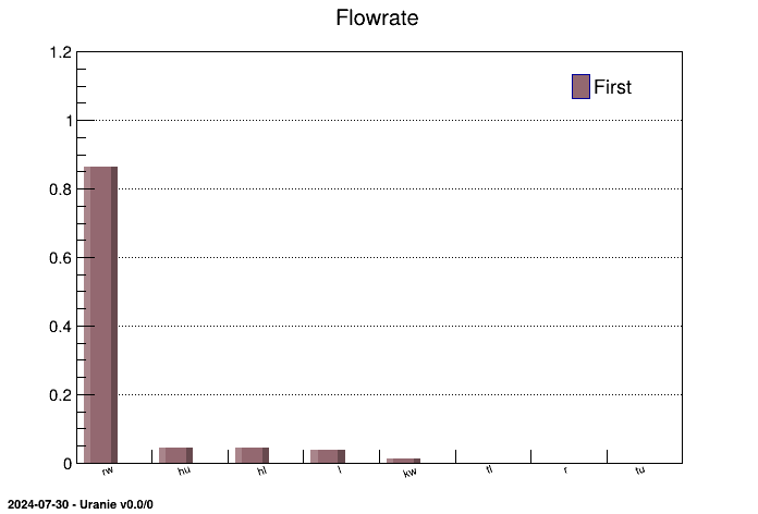
tjrw->drawIndexes("Flowrate", "", "nonewcanv,hist,first");
cc->Print("appliUranieFlowrateJohnsonRW1000Histogram.png");
TCanvas *ccc = new TCanvas("canpie", "TPie");
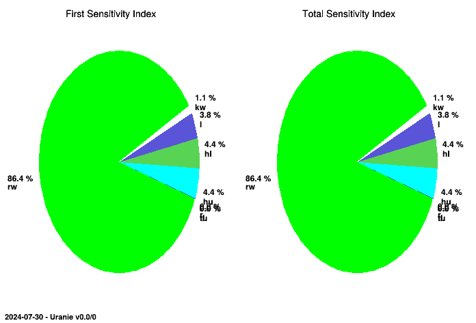
tjrw->drawIndexes("Flowrate", "", "nonewcanv,pie");
ccc->Print("appliUranieFlowrateJohnsonRW1000Pie.png");
}
The figures resulting from this script are shown below and display the sensitivity indices in a histogram and in a
pie chart. The structure of both plots and tables, as they are common with the rest of the sensitivity class,
provides the results in the ntuple that can be reached with getResultTuple(). This
explains why the results are stored in the Sobol column.
First, define the uncertain parameters and add them to a TDataServer object:
// Define the DataServer
TDataServer *tds = new TDataServer("tdsflowreate", "DataBase flowreate");
tds->addAttribute( new TUniformDistribution("rw", 0.05, 0.15));
tds->addAttribute( new TUniformDistribution("r", 100.0, 50000.0));
tds->addAttribute( new TUniformDistribution("tu", 63070.0, 115600.0));
tds->addAttribute( new TUniformDistribution("tl", 63.1, 116.0));
tds->addAttribute( new TUniformDistribution("hu", 990.0, 1110.0));
tds->addAttribute( new TUniformDistribution("hl", 700.0, 820.0));
tds->addAttribute( new TUniformDistribution("l", 1120.0, 1680.0));
tds->addAttribute( new TUniformDistribution("kw", 9855.0, 12045.0));
There are four different kinds of constructors to build a TJohnsonRW object, each corresponding to a different problem:
- the model is either provided data or just a correlation matrix;
- the model is an analytic function run by Uranie,
- the model is a code run by Uranie.
- the model is either a function or a code and the problem is specified through a Relauncher architecture.
The constructor prototype used when data are provide (or one will not used data but just a correlation matrix):
// Create a TJohnsonRW object data
TJohnsonRW(TDataServer *tds, const char *inp,  const char *out ,  const char *Option="")
This constructor takes up to four arguments:
- a pointer to a
TDataServerobject, - a string to specify the names of the input factors separated by ':' (ex. "rw:r:tu:tl:hu:hl:l:kw"), no default is accepted,
- a string to specify the names of the output variables of the model, no default is accepted.
- a string to specify the options, by default empty "";
Here is an example of how to use the constructor with provided data:
TJohnsonRW * tjrw = new TJohnsonRW(tds, "rw:r:tu:tl:hu:hl:l:kw", "flowrateModel"); The way to inject the correlation matrix is discussed below.
The constructor prototype used with an analytic function is:
// Create a TJohnsonRW object with an analytic function
TJohnsonRW(TDataServer *tds,  void *fcn,  const char *inp,  const char *out,  Int_t ns)
TJohnsonRW(TDataServer *tds,  const char *fcn,  Int_t ns,  const char *inp="",  const char *out="")
This constructor takes five arguments:
- a pointer to a
TDataServerobject, - a pointer to an analytic function (either a
voidor aconst charthat represents the function's name when it has been loaded in ROOT's memory), - an integer to specify the number of simulations, its default value is 100,
- a string to specify the names of the input factors separated by ':' (ex. "rw:r:tu:tl:hu:hl:l:kw"), its default value might be the empty string "",
- a string to specify the names of the output variables of the model, its default value might be the empty string "".
Here is an example of how to use the constructor with an analytic function:
Int_t nS = 50;
TJohnsonRW * tjrw_func = new TJohnsonRW(tds, "flowrateModel", nS, "rw:r:tu:tl:hu:hl:l:kw", "flowrateModel"); The constructor prototype used with a code is:
// Create a TJohnsonRW object with a code
TJohnsonRW(TDataServer *tds, TCode *fcode,  Int_t ns, Option_t *option="")
This constructor takes three arguments:
- a pointer to a
TDataServerobject, - a pointer to a
TCode, - an integer to specify the number of simulations.
Here is an example of the use of this constructor on the flowrate case:
// The reference input file
TString sJDDReference = TString("flowrate_input_with_keys.in");

// Set the reference input file and the key for each input attributes
tds->getAttribute("rw")->setFileKey(sJDDReference, "Rw");
tds->getAttribute("r")->setFileKey(sJDDReference, "R");
tds->getAttribute("tu")->setFileKey(sJDDReference, "Tu");
tds->getAttribute("tl")->setFileKey(sJDDReference, "Tl");
tds->getAttribute("hu")->setFileKey(sJDDReference, "Hu");
tds->getAttribute("hl")->setFileKey(sJDDReference, "Hl");
tds->getAttribute("l")->setFileKey(sJDDReference, "L");
tds->getAttribute("kw")->setFileKey(sJDDReference, "Kw");

// The output file of the code
TOutputFileRow *fout = new TOutputFileRow("_output_flowrate_withRow_.dat");
// The attribute in the output file
fout->addAttribute(new TAttribute("yhat"));

// Instanciation de mon code
TCode *mycode = new TCode(tds, "flowrate -s -k");
// Adding the outputfile to the tcode object
mycode->addOutputFile( fout );

// Size of a sampling.
Int_t nS2 = 50;
TJohnsonRW * tjrw2 = new TJohnsonRW(tds, mycode, nS2); The constructor prototype used with a runner is:
// Create a TJohnsonRW object with a runner
TJohnsonRW(TDataServer *tds, TRun *frun,  Int_t ns, Option_t *option="")
This constructor takes three arguments:
- a pointer to a
TDataServerobject, - a pointer to a
TRun, - an integer to specify the number of simulations.
Here is an example of the use of this constructor on the flowrate code in sequential mode:
// The input file
TKeyScript infile("flowrate_input_with_keys.in");
// provide the input and their key
infile.setInputs(8, tds->getAttribute("rw"), "Rw", tds->getAttribute("r"), "R",
tds->getAttribute("tu"), "Tu", tds->getAttribute("tl"), "Tl", tds->getAttribute("hu"), "Hu",
tds->getAttribute("hl"), "Hl", tds->getAttribute("l"), "L", tds->getAttribute("kw"), "Kw");

TAttribute yhat("yhat");
// The output file of the code
TKeyResult outfile("_output_flowrate_withKey_.dat");
// The attribute in the output file
outfile.addOutput(&yhat, "yhat");

// Instanciation de mon code
TCodeEval code("flowrate -s -k");
// Adding the intput/output file to the code
code.addInputFile(&infile);
code.addOutputFile(&outfile);

TSequentialRun run(&code);
run.startSlave();
if(run.onMaster())
{
    // Size of a sampling.
    Int_t nS2 = 50;
    TJohnsonRW * tjrwR = new TJohnsonRW(tds, &run, nS2);
    //...
}
With the Johnson relative weight method, it is possible to use either data loaded from an existing file or no data
at all but only corration matrix to estimate the weights and the  . This former is done, as usual, by calling the
fileDataRead of the TDataserver object. This is not
discussed in details as these as this aspect if fairly classical. The later on the other hand, is new and specific
to the TJohnsonRW class. This possibility is very specific and can be used through the
method setCorrelationMatrix(TMatrixD Corr);
Warning
It is important to pay attention not to mix up
setInputCorrelationMatrix, setCorrelationMatrix. The former is
useful to generate a correlated sample before submitting the computation with function or code (see Section VI.7.1.5 for instance) while the latter is a correlation matrix that does not only contains
the input variables but also the output ones.
Here is an exemple of code that shows how to use this possibility. It starts with the input attribute definition
(using StochasticAttributes is not compulsory anymore has no design-of-experiments will be drawn), along
with the output ones. Once done, the full correlation matrix (inputs and outputs) can be provided through the
setCorrelationMatrix() (for more details on the GenCorr method,
see Section XIV.5.18.2). The rest is pretty much
straightforward.
// Load the GenCorr function
gROOT->LoadMacro("UserFunctions.C");

// Define the DataServer
TDataServer *tds = new TDataServer("tdsflowrate", "Ex. Flowrate");
tds->addAttribute("rw");
tds->addAttribute("r");
tds->addAttribute("tu");
tds->addAttribute("tl");
tds->addAttribute("hu");
tds->addAttribute("hl");
tds->addAttribute("l");
tds->addAttribute("kw");
// outputs
tds->addAttribute("flowrateModel");
tds->getAttribute("flowrateModel")->setOutput();

// Get the full correlation matrix
TMatrixD inCorr(8,8); //Input size definition
GenCorr(&inCorr, true, true);
// inCorr is now 9 by 9 as linearOutput has been added in GenCorr

TJohnsonRW * tjrw = new TJohnsonRW(tds, "rw:r:tu:tl:hu:hl:l:kw", "flowrateModel");
tjrw->setCorrelationMatrix(inCorr);
tjrw->computeIndexes();
To generate the sample that can be used to get the relative weights, one can use the
generateSample method defined in TSensitivity but the purpose of the
relative weight method is focusing on correlated inputs issue. In order to do this, one should specify the
correlation structure of the inputs through the method setInputCorrelationMatrix(TMatrixD
Corr) where the only argument is a correlation matrix that has to be a symmetrical positive definite
matrix whose coefficients have to be in  while the diagonal ones must be set to 1. With the usual variable
definition, this could look like this:
while the diagonal ones must be set to 1. With the usual variable
definition, this could look like this:
TMatrixD inCorr(8,8);
double corrValue[64]={1,0.184641,-0.613412,-0.214481,0.373538,-0.0926293,0.656586,0.194991,
  0.184641,1,0.134385,0.0704593,-0.284958,0.105629,-0.536972,0.663751,
  -0.613412,0.134385,1,0.200747,-0.174041,0.0817216,-0.547402,0.0202687,
  -0.214481,0.0704593,0.200747,1,-0.128116,-0.248905,-0.263717,-0.0613039,
  0.373538,-0.284958,-0.174041,-0.128116,1,-0.0832623,0.397725,-0.675141,
  -0.0926293,0.105629,0.0817216,-0.248905,-0.0832623,1,0.111711,0.100442,
  0.656586,-0.536972,-0.547402,-0.263717,0.397725,0.111711,1,-0.302142,
  0.194991,0.663751,0.0202687,-0.0613039,-0.675141,0.100442,-0.302142,1};
inCorr.Use(8,8,corrValue);

//Create the jrw object
TJohnsonRW * tjrw = new TJohnsonRW(tds, "flowrateModel", nS, "rw:r:tu:tl:hu:hl:l:kw", "flowrateModel");
tjrw->setInputCorrelationMatrix(inCorr);
tjrw->generateSample();
Then, the sample generated can be exported in a file and used outside of Uranie to compute the simulations associated.
To compute the indices, run the method computeIndexes:
tjrw->computeIndexes();Note that this method is all inclusive: it constructs the sample, launches the simulations and computes the indices.
To display graphically the coefficients, use the method drawIndexes:
void TSensitivity::drawIndexes(TString sTitre, const char *select, Option_t * option)The method needs:
- a
TStringcontaining the title of the figure, - a string containing a selection (empty if no selection),
- a string containing the options of the graphics separated by commas.
Some of the options available are:
- "nonewcanv": to not create a new canvas,
- "pie": to display a pie chart,
- "hist": to display a histogram,
- "first": to display the indices of the first order (with "hist" only),
In our example the use of this method is:
TCanvas *cc = new TCanvas("canhist", "histogramme");
tjrw->drawIndexes("Flowrate", "", "nonewcanv,hist,first");
cc->Print("appliUranieFlowrateJohnsonRW500Histogram.png");

TCanvas *ccc = new TCanvas("canpie", "TPie",5,64,1270,560);
tjrw->drawIndexes("Flowrate", "", "nonewcanv,pie");
ccc->Print("appliUranieFlowrateJohnsonRW500Pie.png");
The coefficients, once computed, are stored in a TTree. To get this
TTree, use the method TSensitivity::getResultTuple():
TTree * results = tjrw->getResultTuple();
Several methods exist in ROOT to extract data from a TTree, it is advised to look for them
into the ROOT documentation. We propose two ways of extracting the value of each coefficient from the
TTree.
The method use the method getValue of the TJohnsonRW object specifying the
order of the extract value ("First"), the related input and possibly more selected options.
double hl_first_index = tjrw->getValue("First","hl");The second method uses 3 steps to extract an index:
-
scan the
TTreefor the chosen input variable (with a selection) in order to obtain its row number. In our example, if we chose the variable "hl", we'll use the command:
and in the resulting figure below we see that the first order index of "hl" is in the row 10:results->Scan("*","Inp==\"hl\"");************************************************************************* * Row * Out * Inp * Order * Method * Algo * Value * ************************************************************************* * 10 * flowrateM * hl * First * Johnso * --first-- * 0.0435594 * * 11 * flowrateM * hl * Total * Johnso * --total-- * 0.0435594 * *************************************************************************
-
set the entry of the
TTreeon this row with the methodGetEntry; -
get the value of the index with
GetValuemethod on the "Value" leaf of theTTree.
Below is an example of extraction of the index for "hl" in our flowrate case:
results->Scan("*","Inp==\"hl\"");
results->GetEntry(100);
Double_t S_Rw_Indexe = results->GetLeaf("Value")->GetValue(); The third method uses 2 steps to extract an index:
-
use the
Drawmethod with a selection to select the index, for example the selection for the first order index of "rw" is "Inp==\"rw\" && Algo==\"--first--\""; -
get the pointer on the value of the index with
GetV1method on theTTree.
Below is another example of extraction of the first order index for "rw" in our flowrate case:
results->Draw("Value","Inp==\"rw\" && Algo==\"--first--\"","goff");
Double_t S_Rw_IndexeS = results->GetV1()[0];
Summary: TJohnsonRW methods
setInputCorrelationMatrix(TMatrixD inCorr): define the correlation matrix that is used to intricate the input variables one to another.- inCorr: a
 symmetrical positive definite matrix whose coefficients should
all be in but the diagonal ones which should be set to 1.
symmetrical positive definite matrix whose coefficients should
all be in but the diagonal ones which should be set to 1.
- inCorr: a
setCorrelationMatrix(TMatrixD Corr): define the global correlation matrix that is used to intricate the input and output variables one to another.- Corr: a symmetrical positive definite matrix whose
coefficients should all be in but the diagonal ones which should be set to 1.
- Corr: a
generateSample(Option_t *option=""): generate the sample used for computing the sensitivity indices.- option: no option has been implemented
computeIndexes(Option_t *option=""): compute the Sobol sensitivity indices.- option: string specifying the drawIndexes option used .
void
drawIndexes(TStringsTitre, const char* select="", Option_t *option=""): draw the coefficients.- sTitre: a string containing the title of the figure.
- select: a string containing a solution.
- option: a string containing the options of the graphics separated by commas.
| |  | |
| VI.6. Fourier-based methods |  | VI.8. Sensitivity Indices based on HSIC |