

Documentation
/ Manuel utilisateur en Python
: 
| V.3. Chaos polynomial expansion | ||
|---|---|---|
 | Chapter V. The Modeler module |  |
The basic idea of chaos polynomial expansion (later referred to as PC ) is that any
square-integrable function can be written as 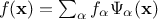 where
where  are the PC coefficients,
  is the orthogonal polynomial-basis. The index over which the sum is done,
 , corresponds to a
multi-index whose dimension is equal to the dimension of vector
, corresponds to a
multi-index whose dimension is equal to the dimension of vector  (i.e.
(i.e.  ) and whose L1 norm (
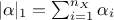 ) is the degree of the resulting
polynomial. More theoretical discussion can be found on this in [metho].
) is the degree of the resulting
polynomial. More theoretical discussion can be found on this in [metho].
In Uranie only a certain number of laws can be used and they have their own preferred orthogonal polynomial-basis. The association of the law and the polynomial basis is show in Table V.2. This association is not compulsory, as one can project any kind of law on a polynomial basis which will not be the best-suited one, but the very interesting interpretation of the coefficients will then not be meaningful anymore.
Table V.2. List of best adapted polynomial-basis to develop the corresponding stochastic law
| Distribution \ Polynomial type | Legendre | Hermite | Laguerre | Jacobi |
|---|---|---|---|---|
| Uniform | X | |||
| LogUniform | X | |||
| Normal | X | |||
| LogNormal | X | |||
| Exponential | X | |||
| Beta | X |
Presentation of the test cases
The Ishigami function is usually used as a "benchmark" in the domain of sensitivity because we
are able to calculate the exact values of the sensitivity index (discussed in Chapter VI
and in [metho]). This function is defined by the following equation:

where the  follow a uniform
distribution on
follow a uniform
distribution on  ,
and A, B are constants. We take A=7, B=0.1 (as done in [ishigami1990importance]).
,
and A, B are constants. We take A=7, B=0.1 (as done in [ishigami1990importance]).
The wrapper of the Nisp library, Nisp standing for Non-Intrusive Spectral Projection, is a tool allowing to access to Nisp functionality from the Uranie platform. The main features are detailed below.
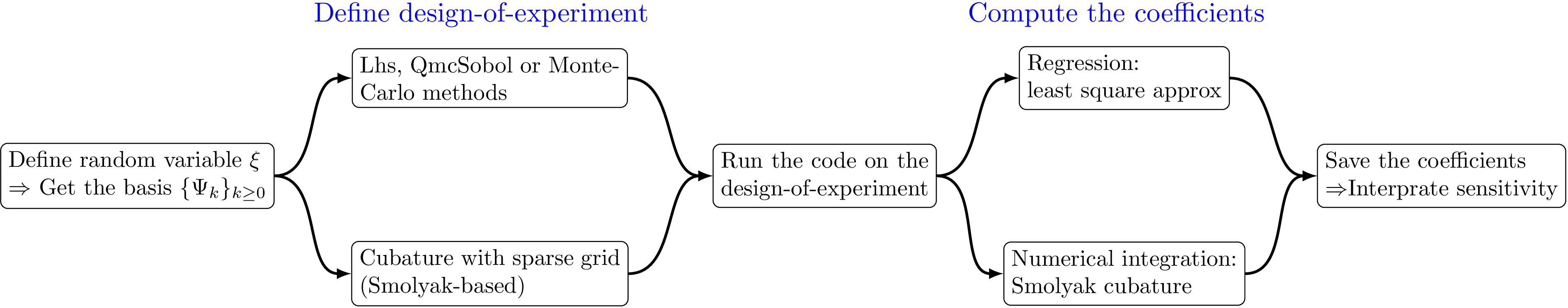
The Nisp library [baudininria-00494680] uses spectral methods based on polynomial chaos in order to provide a surrogate model and allow the propagation of uncertainties if they arise in the numerical models. The steps of this kind of analysis, using the Nisp methodology are represented schematically in Figure V.2 and are introduced below:
Specification of the uncertain parameters xi,
Building stochastic variables associated xi,
Building a design-of-experiments
Building a polynomial chaos, either with a regression or an integration method (see Section V.3.1.1 and Section V.3.1.1)
Uncertainty and sensitivity analysis
The regression method is simply based on a least-squares approximation: once the design-of-experiments is done, the vector of
output  is
computed with the code. By writing the correspondence matrix
is
computed with the code. By writing the correspondence matrix
 and the
coefficient-vector
and the
coefficient-vector  , this estimation is just a minimisation of
  . As
already stated in Section V.2, this leads to write the general form of the solution
as
. As
already stated in Section V.2, this leads to write the general form of the solution
as 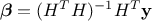 which also shows that the way the design-of-experiments is performed can be optimised
depending on the case under study (and might be of the utmost importance in some rare case).
which also shows that the way the design-of-experiments is performed can be optimised
depending on the case under study (and might be of the utmost importance in some rare case).
In order to perform this estimation, it is mandatory to have more points in the design-of-experiments than the number of
coefficient to be estimated (in principle, following the rule 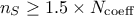 leads to a safe estimation). For more information on this method, see [metho].
The integration method relies on a more "complex" design-of-experiments. It is indeed recommended to have dedicated design-of-experiments, made
with a Smolyak-based algorithms (as the ones cited in Figure V.2). These design-of-experiments are
sparse-grids and usually have a smaller number of points than the regularly-tensorised approaches. In this case,
the number of samples has not to be specified by the user. Instead, the argument requested describes the level of
the design-of-experiments (which is closely intricated, as the higher the level is, the larger the number of samples is). Once this
is done, the calculation is performed as a numerical integration by quadrature methods, which requires a large
number of computations.
In the case of Smolyak algorithm, this number can be expressed by the number of
dimensions and the requested
level  as
as  which shows an
improvement with respect to the regular tensorised formula for quadrature (
which shows an
improvement with respect to the regular tensorised formula for quadrature ( ).
).
First, it is necessary to build a dataserver containing the uncertain parameters . These parameters are represented by random variables which
follow one of these statistical laws given in Table V.2.[4]
Example:
Within the framework of our case-test example, we are going to build a TDS containing 3 attributes which follow a
uniform law on the interval .
import math
tds = DataServer.TDataServer("tdsishigami", "Ex. Ishigami")
tds.addAttribute(DataServer.TUniformDistribution("x1", -1*math.pi, math.pi))
tds.addAttribute(DataServer.TUniformDistribution("x2", -1*math.pi, math.pi))
tds.addAttribute(DataServer.TUniformDistribution("x3", -1*math.pi, math.pi))
Now, it is necessary to build the stochastic variables  associated to the uncertain parameters specified above. For that, we create a
TNisp object from a TDataServer object by using the constructor TNisp(TDataServer *tds). This constructor builds automatically
attributes representing the stochastic variables from the information contained in the tds.
Explanation:
Families of orthogonal polynomials are automatically associated to the attributes representing the uncertain
parameters . Given the type of
expected law, the corresponding orthogonal polynomial family will be used (as already spotted in Table V.2). However, Uranie gives the possibility to change the family of orthogonal polynomials
associated by default to an attribute. It is then necessary to modify, if needed, at the TNisp
call level, the type of polynomial (by using getStochasticBasis of the
TDataServer library) in order to have the stochastic variables represented by attributes following the chosen law.
Example:
In our example, we do not modify the type of the orthogonal polynomials. Then we call, at once, the constructor
TNisp.
# Define of TNisp object
nisp = Modeler.TNisp(tds)
The stochastic variables are represented by 3 internal attributes following a uniform law on [0,1]. A print of the
TNisp object contents, by using the method printLog, gives the listing below:
** TNisp::printLog[]
   Number of simulation :1
   Number of variable   :3
   Level                :0
   Stochastic variables:
		 -->psi_x1: Uniforme 0 1
	      -->psi_x2: Uniforme 0 1
	      -->psi_x3: Uniforme 0 1
	      Uncertain variables:
	      -->x1: Uniforme -3.14159 3.14159
	      -->x2: Uniforme -3.14159 3.14159
	      -->x3: Uniforme -3.14159 3.14159
fin of TNisp::printLog[]
Now, it is necessary to generate and evaluate the sample.
There are two different ways to generate the sample:
Using the
generateSamplefunctionality of the library NispUsing the Sampler library of Uranie
The Nisp library permits to build a sample thanks to the generateSample(TString method,Int_t n) method. The parameter
n represents the level or the size of the sampler depending on the chosen methodology. The
parameter method represents the building methodology of the sampler. The methods offered by
Nisp are the following:
Table V.3. Methods of sampler generation
| Name of the method | Size | Level |
|---|---|---|
| Lhs | X | |
| Quadrature | X | |
| MonteCarlo | X | |
| SmolyakFejer | X | |
| SmolyakTrapeze | X | |
| SmolyakGauss | X | |
| SmolyakClenchawCurtis | X | |
| QmcSobol | X | |
| Petras | X |
Example:
Within the framework of our test case, we build a sampler of type Petras of level 8.
level = 8
nisp.generateSample("Petras", level)To build a sample using the Sampler library, see Chapter III.
Once the sample has been built, it is necessary to transfer it to the TNisp object. To do
that, we use the setSample(TString "method",Option_t
*option) method where the parameter method is the type of the method
used by the library Sampler and the optional parameter option is the keyword
"savegvx" to use if one wants to save the in the TDataServer.
Below is an example using the functionality:
nombre_simulations = 100
fsampling = Sampler.TSampling(tds, "lhs", nombre_simulations)
fsampling.generateSample()

nisp.setSample("Lhs")
Given that we have the set (uncertain parameter, stochastic variables and sampler), we can build a
TPolynomialChaos object by means of the constructor TPolynomialChaos(TDataServer *tds, TNisp *nisp).
# build a polynomial chaos
pc = Modeler.TPolynomialChaos(tds, nisp)
One can calculate the coefficients of these polynomials with the computeChaosExpansion(TString method) method where the parameter
method is either the keyword Integration or the keyword
Regression.
Example:
Within the framework of our example, we use the "Integration" method.
degree = 8
pc.setDegree(degree)
pc.computeChaosExpansion("Integration")Now, we can do the uncertainty and sensitivity analyses. With the Nisp library, we have access to these following functionality:
Mean:
getMean( ) where parameter is either the name or the index of the output variable,
SVariance:
getVariance() where parameter is either the name or the index of the output variables,
Co-variance:
getCovariance( ,
,  ) where parameters and are either the names or the indexes of the output variables,
Correlation:
getCorrelation(, ) where parameters and are either the names or the indexes of the output variable,
Index of the first order sensitivity
getIndexFirstOrder(, ) where parameter is the name or the index of the input variable and the parameter is the name or the index of the output variable,
Index of total sensitivity:
getIndexTotalOrder(, ) where parameter is the name or the index of the input variable and the parameter is the name or the index of the output variable,
Example:
Within the framework of our example, the instructions are the following:
# Uncertainty and sensitivity analysis
print("Variable Ishigami ================")
print("Mean     = %g " % (pc.getMean("Ishigami")))
print("Variance = %g " % (pc.getVariance("Ishigami")))
print("First Order[1] = %g " % (pc.getIndexFirstOrder("x1","Ishigami")))
print("First Order[2] = %g " % (pc.getIndexFirstOrder("x2","Ishigami")))
print("First Order[3] = %g " % (pc.getIndexFirstOrder("x3","Ishigami")))
print("First Order[1] = %g " % (pc.getIndexTotalOrder("x1","Ishigami")))
print("First Order[2] = %g " % (pc.getIndexTotalOrder("x2","Ishigami")))
print("First Order[3] = %g " % (pc.getIndexTotalOrder("x3","Ishigami")))
The following lines are obtained in the terminal:
Variable Ishigami ================
Mean     = 3.5
Variance = 13.8406
First Order[1] = 0.313997
First Order[2] = 0.442386
First Order[3] = 6.50043e-07
Total Order[1] = 0.557568
Total Order[2] = 0.442477
Total Order[3] = 0.24357
There are other Nisp functionalities accessible from Uranie:
Auto-determination of the degree
Recently a new possibility has been introduced in order to be more efficient and less model dependant when considering the regression procedure. It is indeed possible to ask for an automatic
determination of the best polynomial degree possible. In order to do so, the maximum polynomial degree allowed is
computed using the rule of thumb defined above, and the method computeChaosExpansion is
called with the option "AutoDegree". A polynomial chaos expansion is done from a minimum degree value (one per
default, unless otherwise specified thanks to the setAutoDegreeBoundaries method) up to the
maximum allowed value. To compare the results one to another and be able to decide which one is the best, a
Leave-One-Out method (LOO, which consists in the prediction of a value for using the rest of the known values in the training basis,
i.e.  for
for  ) and the total Mean Square
Error (MSE) are used as estimator. These notions are better introduced in [metho]. The best estimated
degree is evaluated and the polynomial chaos expansion is re-computed, but all results (LOO, MSE...) are stored for
all the considered degrees.
) and the total Mean Square
Error (MSE) are used as estimator. These notions are better introduced in [metho]. The best estimated
degree is evaluated and the polynomial chaos expansion is re-computed, but all results (LOO, MSE...) are stored for
all the considered degrees.
This possibility comes with a bunch of new function implemented to modify the behaviour by default. The basic
configuration is to start with a degree one polynomial expansion and to scan up to a certain degree  that would still satisfy this rule of
thumb
that would still satisfy this rule of
thumb
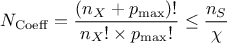
 being a normalisation factor chosen to be 1.5.
The usable methods are listed below:
being a normalisation factor chosen to be 1.5.
The usable methods are listed below:
setAutoDegreeFactor(double autodeg): change the value of the factor for the auto normalisation (not
recommended). The provided number should be greater than one.
setAutoDegreeBoundaries(int amin, int amax): change the degree boundaries from one to amin and, if amax is provided, from the level determined by the automatic procedure described above to the chosen amax value. If amax is greater than the automatic determined limit, the default is not changed.
Save data
It is possible to save polynomial chaos data in a f.dat file with the save(TString sfile) method where sfile is the name of the data
file. This file will contains the following data:
stochastic dimension,
type of the orthogonal polynomial (Legendre, Laguerre or Hermite),
the degree of the polynomial chaos,
the number of polynomial chaos coefficients,
the number of output,
a list of the coefficient values where the first element is the the mean of the output.
# Save the polynomial chaos
pc.save("NispIshigami.dat")
Here is a file .dat corresponding to our example:
nx= 3 Legendre Legendre Legendre no= 8 p= 164 ny= 1 Coefficients[1]= 3.500000e+00 1.625418e+00 2.962074e-17
-2.589041e-17 1.575324e-15 5.233520e-17 -3.175950e-18 -5.947228e-01 -1.278829e-17 1.354792e-15 -1.290638e+00
-1.858390e-18 5.947865e-18 4.838275e-16 8.497435e-18 1.372419e+00 -1.722653e-19 1.330604e-17 -1.575058e-17
5.159489e-18 -1.604235e-15 -1.386085e-17 7.823196e-18 -5.101110e-16 1.268601e-17 1.724496e-17 -1.606472e-17
3.412272e-18 1.035117e-17 1.366688e-18 -1.952291e+00 1.603873e-17 1.960259e-16 9.769466e-18 -5.051477e-16
1.949287e-01 5.167621e-17 2.218591e-17 -3.783569e-17 1.636383e-17 -1.089702e+00 2.653437e-18 1.820189e-17
-3.300252e-17 -1.109147e-17 2.613944e-17 -3.982929e-17 -2.644820e-16 -4.711621e-18 4.091730e-01 5.633658e-17
3.207523e-17 8.469377e-18 -1.623212e-17 -5.221323e-18 -1.348604e-17 -2.549941e-03 -1.380621e-17 4.408383e-18
2.216698e-16 1.055488e-17 -5.971197e-16 -1.077924e-17 -7.500053e-18 -1.398875e-18 8.323369e-18 -1.828664e-16
-1.891202e-17 2.846158e-17 1.240056e-18 -7.184406e-17 -4.183157e-17 1.999887e-17 -1.078061e-17 1.320948e-18
4.955143e-20 6.740688e-18 1.357408e+00 -1.599643e-17 -3.404927e-16 -3.826895e-18 -1.184481e-16 1.175915e-17
-2.549941e-03 -1.266838e-02 4.550685e-17 1.601655e-17 1.855980e-16 1.171108e-17 1.632677e-01 3.035872e-17
-4.384243e-18 -3.127246e-17 1.740356e-17 -3.455894e-19 3.372673e-18 -3.556473e-16 -9.162355e-18 -3.247428e-01
4.190780e-17 -1.547995e-17 -5.808814e-17 9.922144e-18 2.618348e-17 7.213333e-18 -5.300321e-06 -4.983518e-18
-3.503280e-16 -6.190117e-18 3.713020e-16 1.065906e-17 -5.448912e-06 3.825624e-18 1.359954e-17 -7.719858e-18
-1.803757e-18 4.289915e-17 -1.214645e-18 5.479922e-17 -3.330110e-18 1.579483e-03 2.670695e-18 9.359714e-19
2.512771e-02 2.635458e-17 2.622223e-16 -1.309301e-18 8.084506e-18 -1.189488e-17 -4.330879e-18 1.247133e-15
-1.863642e-17 2.096038e-16 -2.331035e-18 3.034432e-16 -1.363808e-17 -3.762944e-18 -1.524500e-17 -8.487270e-19
-1.420178e-17 -4.964460e-18 5.812476e-16 2.572312e-17 -2.088466e-17 1.795371e-17 2.011599e-16 1.878423e-17
1.608204e-15 2.092277e-17 1.776101e-17 -5.185917e-17 -3.704922e-18 -7.070417e-17 2.010136e-17 2.640413e-17
9.647070e-18 -3.393909e-01 -2.530162e-17 8.354699e-16 -1.223963e-18 6.813105e-16 -1.721674e-17 2.512771e-02
9.392854e-18 1.579483e-03
Saving the macro
It is possible to save the problem in a C macro with the exportFunction(char
*sfile,char *sfunction) method where sfile is the name of the .C file and sfunction is the
name of the macro.
# Save the pv in a program (C langage)
pc.exportFunction("NispIshigami", "NispIshigami")
Here is the NispIshigami.C file corresponding to our example:
#include <math.h>

double NispIshigami_beta[1][165]={
3.5,1.62542,2.96207e-17,-2.58904e-17,1.57532e-15,5.23352e-17,-3.17595e-18,-0.594723,
-1.27883e-17,1.35479e-15,-1.29064,-1.85839e-18,5.94787e-18,4.83828e-16,8.49743e-18,1.37242,
-1.72265e-19,1.3306e-17,-1.57506e-17,5.15949e-18,-1.60424e-15,-1.38608e-17,7.8232e-18,
-5.10111e-16,1.2686e-17,1.7245e-17,-1.60647e-17,3.41227e-18,1.03512e-17,1.36669e-18,
-1.95229,1.60387e-17,1.96026e-16,9.76947e-18,-5.05148e-16,0.194929,5.16762e-17,2.21859e-17,
-3.78357e-17,1.63638e-17,-1.0897,2.65344e-18,1.82019e-17,-3.30025e-17,-1.10915e-17,
2.61394e-17,-3.98293e-17,-2.64482e-16,-4.71162e-18,0.409173,5.63366e-17,3.20752e-17,
8.46938e-18,-1.62321e-17,-5.22132e-18,-1.3486e-17,-0.00254994,-1.38062e-17,4.40838e-18,
2.2167e-16,1.05549e-17,-5.9712e-16,-1.07792e-17,-7.50005e-18,-1.39887e-18,8.32337e-18,
-1.82866e-16,-1.8912e-17,2.84616e-17,1.24006e-18,-7.18441e-17,-4.18316e-17,1.99989e-17,
-1.07806e-17,1.32095e-18,4.95514e-20,6.74069e-18,1.35741,-1.59964e-17,-3.40493e-16,
-3.82689e-18,-1.18448e-16,1.17591e-17,-0.00254994,-0.0126684,4.55068e-17,1.60165e-17,
1.85598e-16,1.17111e-17,0.163268,3.03587e-17,-4.38424e-18,-3.12725e-17,1.74036e-17,
-3.45589e-19,3.37267e-18,-3.55647e-16,-9.16236e-18,-0.324743,4.19078e-17,-1.548e-17,
-5.80881e-17,9.92214e-18,2.61835e-17,7.21333e-18,-5.30032e-06,-4.98352e-18,-3.50328e-16,
-6.19012e-18,3.71302e-16,1.06591e-17,-5.44891e-06,3.82562e-18,1.35995e-17,-7.71986e-18,
-1.80376e-18,4.28991e-17,-1.21465e-18,5.47992e-17,-3.33011e-18,0.00157948,2.67069e-18,
9.35971e-19,0.0251277,2.63546e-17,2.62222e-16,-1.3093e-18,8.08451e-18,-1.18949e-17,
-4.33088e-18,1.24713e-15,-1.86364e-17,2.09604e-16,-2.33103e-18,3.03443e-16,-1.36381e-17,
-3.76294e-18,-1.5245e-17,-8.48727e-19,-1.42018e-17,-4.96446e-18,5.81248e-16,2.57231e-17,
-2.08847e-17,1.79537e-17,2.0116e-16,1.87842e-17,1.6082e-15,2.09228e-17,1.7761e-17,
-5.18592e-17,-3.70492e-18,-7.07042e-17,2.01014e-17,2.64041e-17,9.64707e-18,-0.339391,
-2.53016e-17,8.3547e-16,-1.22396e-18,6.81311e-16,-1.72167e-17,0.0251277,9.39285e-18,
0.00157948
};
int NispIshigami_indmul[165][3]={
0,0,0,1,0,0,0,1,0,0,0,1,2,0,0,1,1,0,1,0,1,0,2,0,0,1,1,0,0,2,3,0,0,2,1,0,2,0,1,1,2,0,1,1,1,
1,0,2,0,3,0,0,2,1,0,1,2,0,0,3,4,0,0,3,1,0,3,0,1,2,2,0,2,1,1,2,0,2,1,3,0,1,2,1,1,1,2,1,0,3,
0,4,0,0,3,1,0,2,2,0,1,3,0,0,4,5,0,0,4,1,0,4,0,1,3,2,0,3,1,1,3,0,2,2,3,0,2,2,1,2,1,2,2,0,3,
1,4,0,1,3,1,1,2,2,1,1,3,1,0,4,0,5,0,0,4,1,0,3,2,0,2,3,0,1,4,0,0,5,6,0,0,5,1,0,5,0,1,4,2,0,
4,1,1,4,0,2,3,3,0,3,2,1,3,1,2,3,0,3,2,4,0,2,3,1,2,2,2,2,1,3,2,0,4,1,5,0,1,4,1,1,3,2,1,2,3,
1,1,4,1,0,5,0,6,0,0,5,1,0,4,2,0,3,3,0,2,4,0,1,5,0,0,6,7,0,0,6,1,0,6,0,1,5,2,0,5,1,1,5,0,2,
4,3,0,4,2,1,4,1,2,4,0,3,3,4,0,3,3,1,3,2,2,3,1,3,3,0,4,2,5,0,2,4,1,2,3,2,2,2,3,2,1,4,2,0,5,
1,6,0,1,5,1,1,4,2,1,3,3,1,2,4,1,1,5,1,0,6,0,7,0,0,6,1,0,5,2,0,4,3,0,3,4,0,2,5,0,1,6,0,0,7,
8,0,0,7,1,0,7,0,1,6,2,0,6,1,1,6,0,2,5,3,0,5,2,1,5,1,2,5,0,3,4,4,0,4,3,1,4,2,2,4,1,3,4,0,4,
3,5,0,3,4,1,3,3,2,3,2,3,3,1,4,3,0,5,2,6,0,2,5,1,2,4,2,2,3,3,2,2,4,2,1,5,2,0,6,1,7,0,1,6,1,
1,5,2,1,4,3,1,3,4,1,2,5,1,1,6,1,0,7,0,8,0,0,7,1,0,6,2,0,5,3,0,4,4,0,3,5,0,2,6,0,1,7,0,0,8
};
void NispIshigami_legendre(double *phi,double x, int no) {
   int i;
   x=2.*x-1.;
   phi[0]=1.; if(no>0)  phi[1]=x;
   for(i=1;i<no;i++)    phi[i+1]= ((2.*i+1.) * x * phi[i] - i * phi[i-1]) / (i+1.);
   for(i=0;i<=no;i++)   phi[i]  = phi[i] * sqrt(2.* i + 1.);
}
void NispIshigami(double *x, double *y)
{
  //////////////////////////////
  //
  //     *********************************************
  //     ** Uranie v2.3/1
  //     ** Export Nisp :
  //     ** Date : Thu Jun 16 15:54:02 2011
  //     *********************************************
  //
  //
  //     *********************************************
  //     ** TDataServer : tdsishigami **
  //     **
  //     ** Ex. Ishigami **
  //     *********************************************
  //
  //
  //////////////////////////////
   int i,j,k,nx,ny,no,p;
   nx=3;ny=1;no=8;p=165;
   double psi[165],phi[3][9],xi[3],s;
   for(i=0;i<nx;i++) xi[i]=x[i];
   NispIshigami_legendre(phi[0],xi[0],8);
   NispIshigami_legendre(phi[1],xi[1],8);
   NispIshigami_legendre(phi[2],xi[2],8);
   for(k=0;k<=p;k++) {
      for(psi[k]=1.,i=0;i<nx;i++) psi[k]=psi[k]*phi[i][NispIshigami_indmul[k][i]];
   }
   for(j=0;j<ny;j++) {
      for(s=0.,k=0;k<=p;k++) s+=NispIshigami_beta[j][k]*psi[k];
      y[j]=s;
   }
}
Index of sensitivity of a group of input variables
It is possible to compute the sensitivity index for a group of input variable for a given output variable.
print("value indice: %g " %(pc.getIndex("x1:x3", "Ishigami")))Within the framework of our example, this results in the following message:
value indice: 0.557523
Index of sensitivity of a group of input variables in interaction
It is possible to compute the sensitivity index for a group of input variable in interaction for a given output variable.
print("value indice: %g " %(pc.getIndexInteraction("x1:x3", "Ishigami")))Within the framework of our example, this leads to the following line in the terminal:
value indice: 0.243525
Recover the various dimensions
It is possible to recover:
the number of input variables with
getDimensionInput(),the number of output variables with
getDimensionOutput()the number of coefficients with
getDimensionExpansion()
print("nx = %d " % (pc.getDimensionInput()))
print("ny = %d " % (pc.getDimensionOutput()))
print("p = %d " % (pc.getDimensionExpansion()))
With our example, this leads to the following line in the terminal:
nx = 3
ny = 2
p = 165
Calculate output values
It is possible to compute the output of a polynomial chaos for a given input vector.
import numpy as np
xi = np.array([0.8, 0.2, 0.7])
pc.computeOutput(xi)
print("Ishigami     =  %g " %(pc.getOutput(0)))
With our example, this leads to the following line in the terminal:
Ishigami = 7.80751
| |  | |
V.2. The TLinearRegression class |  | V.4. Adaptive development in polynomial chaos: the Anisp method |