

Documentation
/ Guide méthodologique
: 
| Chapter VII. The Calibration module | ||
|---|---|---|
 |  | |
Table of Contents
This section presents different calibration methods that are provided to help achieve an accurate estimation of the parameters of a model with respect to data (either from experiment or from simulation). The methods implemented in Uranie are ranging from point estimation to more advanced Bayesian techniques and they mainly differ in the hypotheses they rely on.
In general, a calibration procedure requires an input dataset meaning an existing set of
elements (either resulting from simulations or experiments). This ensemble (of size  ) can be written as
 is the i-th input vector which can be written as
  while
while  is the i-th output vector which can be written as
.
These data
will be compared with model predictions, where the model is a
mathematical function
is the i-th output vector which can be written as
.
These data
will be compared with model predictions, where the model is a
mathematical function  . From now on and unless otherwise specified the
dimension of the output is set to 1 (
. From now on and unless otherwise specified the
dimension of the output is set to 1 ( ) which means
that the reference observations and the predictions of the model are scalars (the observations will then be written
) which means
that the reference observations and the predictions of the model are scalars (the observations will then be written
 and the predictions of the model
 ).
).
In addition to the already introduced previously
input vector, the model also depends on a parameter vector
 which is constant but unknown. The model is deterministic, meaning that is constant once both
  and
and  are fixed. In the rest of this documentation, a given set of parameter values
is called a configuration.
are fixed. In the rest of this documentation, a given set of parameter values
is called a configuration.
The standard hypothesis for probabilistic calibration is that the observations differ from the predictions of the model by a certain amount which is supposed to be a random variable as
where
 is a random
variable whose expectation is equal to 0 and which is called residuals. This variable represents the
deviation between the model prediction and the observation under investigation. It might arise from two possible
origins which are not mutually exclusive:
is a random
variable whose expectation is equal to 0 and which is called residuals. This variable represents the
deviation between the model prediction and the observation under investigation. It might arise from two possible
origins which are not mutually exclusive:
experimental: affecting the observations. For a given observation, it could be written
modelling: the chosen model
 is intrinsically not correct. This contribution could be written
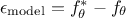
As the ultimate goal is to have 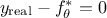 , injecting back the two contributions discussed above, this translates
back to equation Equation VII.1, only breaking down:
, injecting back the two contributions discussed above, this translates
back to equation Equation VII.1, only breaking down: 
The rest of this section introduces two important discussions that will be referenced throughout this module:
the distance between observations and the predictions of the models, in Section VII.1.1;
the theoretical background and hypotheses (linear assumption, concept of prior and posterior distributions, the Bayes formulation...) in Section VII.1.2.
The former is simply the way to obtain statistics over the samples of the reference observations when comparing them to a set of parameters and how
these statistics are computed when the  . The latter is a general introduction, partly reminding elements already introduced in other
sections and discussing some assumptions and theoretical foundations needed to understand the methods discussed later on.
. The latter is a general introduction, partly reminding elements already introduced in other
sections and discussing some assumptions and theoretical foundations needed to understand the methods discussed later on.
On top of this description, there are several predefined calibration procedures proposed in the Uranie platform:
Minimisation techniques in Section VII.2
Analytical linear Bayesian estimation in Section VII.3
Approximate Bayesian Computation techniques (ABC) in Section VII.4
Markov chain Monte Carlo approach in Section VII.5
CIRCE method in Section VII.6
There are many ways to quantify the agreement between the reference observations and the model predictions, given a
parameter vector . Depending on the framework adopted (deterministic or Bayesian), different tools are required. In a
deterministic setting, a distance is used to measure how far the prediction is from the observation. In contrast,
within the Bayesian framework, the analogous concept is the likelihood, a function that evaluates the probability of
observing the data given a parameter vector.
Since the number of variables  used to perform the calibration can be greater than one, it might be useful to introduce the coefficients
 to weight the contribution of each variable relative to the others. The following lists the distance functions available in Uranie:
L1 distance function (sometimes called Manhattan distance):
 ;
;
Least squares distance function:
;
Relative least squares distance function:
 ;
;
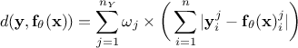
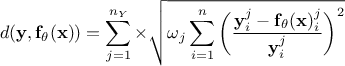
Weighted least squares distance function:
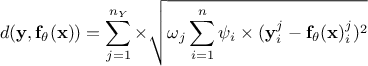 , where the coefficients
 are associated with the j-th variable and are used to weight each observation with respect to the others;
Mahalanobis distance function:
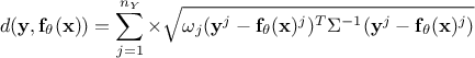 where
where  is the covariance matrix of the observations.
Regarding the likelihood functions already implemented, only the Gaussian log-likelihood for independent parameters is available, as it is the most commonly used. Its expression follows:
Gaussian log-likelihood for independent parameters:
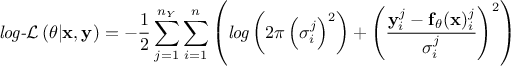 where the
coefficients
where the
coefficients  are the standard deviations of each observation associated to the j-th variable.
If needed, it is still possible to define a custom likelihood (or distance).
These definitions are not orthogonal. Indeed, if 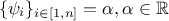 , then the least squares
function is equivalent to the weighted least squares one. This situation is realistic, as it can correspond to the
case where the least squares estimation is weighted with an uncertainty affecting the observations, assuming the
uncertainty is constant throughout the data (meaning
, then the least squares
function is equivalent to the weighted least squares one. This situation is realistic, as it can correspond to the
case where the least squares estimation is weighted with an uncertainty affecting the observations, assuming the
uncertainty is constant throughout the data (meaning  ). This is called the homoscedasticity
assumption and it is important for the linear case, as discussed later on.
). This is called the homoscedasticity
assumption and it is important for the linear case, as discussed later on.
One can also compare the relative and weighted least squares, if  and
and 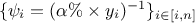 ,these two forms
become equivalent (the relative least squares is useful when uncertainty on observations is multiplicative). Finally, if one
assumes that the covariance matrix of the observations is the identity (meaning
,these two forms
become equivalent (the relative least squares is useful when uncertainty on observations is multiplicative). Finally, if one
assumes that the covariance matrix of the observations is the identity (meaning
 ), the
Mahalanobis distance is equivalent to the least squares distance.
), the
Mahalanobis distance is equivalent to the least squares distance.
Warning
It might seem natural to think that the lower the distance is, the closer our parameters are to the real values. Bearing this in mind would mean thinking that "having a null distance" is the ultimate target of calibration, which is actually dangerous. As for the general discussion in Chapter IV, the risk could be to overfit the set of parameters by "learning" just the set of observations at our disposal as the "truth", not considering that the residuals (introduced in Equation VII.1) might be here to introduce observation uncertainties. In this case, knowing the value of the uncertainty on the observations, the ultimate target of the calibration might be to get the best agreement of observations and model predictions within the model uncertainty, which can be translated into a distribution of the reduced-residuals (that would be something like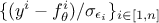 in a scalar case) behaving like a standard
normal distribution.
in a scalar case) behaving like a standard
normal distribution.
VVUQ is a known acronym standing for "Verification, Validation and Uncertainty Quantification". Within this framework, the calibration procedure of a model, sometimes also called "Inverse problem" [Tarantola2005] or "data assimilation" [Asch2016] depending on the assumptions and the context, is an important step of uncertainty quantification. This step should not be confused with validation, even if both procedures are based on a comparison between reference data and model predictions, their definitions are given below [trucano2006calibration]
- validation:
process of determining the degree to which a model is an accurate representation of the real world for its intended uses.
- calibration:
process of improving the agreement between model calculations and a chosen set of benchmarks by adjusting the parameters implemented in the model.
The underlying question of validation is "What is the confidence level that can be granted to the model given the difference seen between the predictions and physical reality ?" while the underlying question of calibration is "Given the chosen model, which parameter value minimises the difference between a set of observations and its predictions, under the chosen statistical assumptions?".
It sometimes happens that a calibration problem allows an infinite number of equivalent solutions
[Hansen1998], which is possible for instance when the chosen model depends explicitly on an operation of two parameters. The simplest
example would be to have a model depending only on two parameters through the difference  . In this peculiar case,
every couple of parameters
. In this peculiar case,
every couple of parameters  that would lead to the same difference would provide the exact same
model prediction, which means that it is impossible to disentangle these solutions. This issue, also known as parameter
identifiability, is crucial as one needs to consider how the chosen model is parameterised
[walter1997identification].
that would lead to the same difference would provide the exact same
model prediction, which means that it is impossible to disentangle these solutions. This issue, also known as parameter
identifiability, is crucial as one needs to consider how the chosen model is parameterised
[walter1997identification].
Defining a calibration analysis consists in several important steps:
Specify the set of observations that will be used as reference;
Specify the model that is supposed to adequately represent the real world;
Define the parameters to be analysed (either by specifying a priori distributions or at least by setting a range). This step requires particular caution concerning identifiability.
Choose the method used to calibrate the parameters.
Choose the distance function used to quantify the discrepancy between the observations and the model predictions.
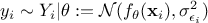
The least squares distance function introduced in Section VII.1.1 is widely used when considering calibration issues. This is true whether calibration is performed within a statistical framework or not (see the discussion on uncertainty sources in Section VII.1). The importance of the least squares approach can be understood by adding an additional assumption on the residuals defined previously. If one considers that the residuals are normally distributed, it implies that one can write

where  can quantify both sources
of uncertainty and whose values are supposed known. The formula above can be used to transform Equation VII.1 into (setting
can quantify both sources
of uncertainty and whose values are supposed known. The formula above can be used to transform Equation VII.1 into (setting  for simplicity):
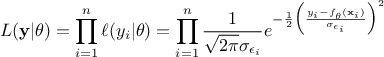
This particular case is very interesting, as from Equation VII.2 it
becomes possible to write down the probability of the observation set  as the product of all its component probabilities which can
be summarised as such:
as the product of all its component probabilities which can
be summarised as such:
It is logical to consider that, since the dataset has been observed, the probability of this collection of observations
must be high. The probability defined in Equation Equation VII.3 can then be
maximised by varying in
order to get its most probable values. This is called the Maximum Likelihood Estimation (MLE) and maximising the
likelihood is equivalent to minimising the logarithm of the likelihood which can be written as:
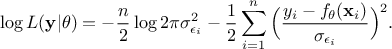
The first part of the right-hand side is independent
of which means that minimising the log-likelihood is basically
focusing on the second part of the right-hand side which essentially corresponds to the weighted least squares distance
with the weights set to 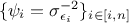 .
.
Their values depend on the underlying model assumptions, and this discussion is postponed to another section (this is discussed in Section VII.2). More details on least squares concepts can be found in many references, such as [Borck1996, Hansen2013].
The probability of an event occurring can be seen as the limit of its occurrence rate or as the quantification of a
personal judgement or opinion regarding its realisation. This is a difference in interpretation that usually distinguishes the
frequentist from the Bayesian perspective. For a simple illustration one can flip a coin: the probability of getting heads,
denoted  is either the average result of a very large number of experiments (this definition is very factual, but its
value depends strongly on the number of experiments) or the personal belief that the coin is well-balanced or not (which
is basically an a priori opinion that might be based on observations, or not).
is either the average result of a very large number of experiments (this definition is very factual, but its
value depends strongly on the number of experiments) or the personal belief that the coin is well-balanced or not (which
is basically an a priori opinion that might be based on observations, or not).
Let's call  a
random vector with a joint probability density
a
random vector with a joint probability density  and marginal densities written as
  and
and  . From there, the Bayes' rule states that:
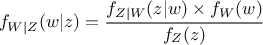
where  (respectively
  ) is the conditional probability density of
 knowing that
  has been realised (and vice-versa
respectively). These laws are called conditional laws.
has been realised (and vice-versa
respectively). These laws are called conditional laws.
Getting back to our formalism introduced previously, using Equation Equation VII.5 implies that
the probability density of the random variable given our observations, which is called posterior
distribution, can be expressed as
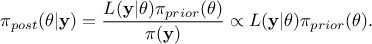
In this equation,  represents the conditional probability of the observations knowing the
values of ,
represents the conditional probability of the observations knowing the
values of ,
 is
the a priori probability density of , often referred to as prior,
is
the a priori probability density of , often referred to as prior,  is the marginal likelihood
of the observations, which is constant in our scope (as it does not depend on the values of but only on its prior, as
is the marginal likelihood
of the observations, which is constant in our scope (as it does not depend on the values of but only on its prior, as  , it consists only in a normalizing factor).
The prior law is said to be proper when one can integrate it, and improper
otherwise. It is conventional to simplify the notations, by writing  instead of
  and
also
and
also  instead of
.
The choice of the prior is a crucial step when defining the calibration procedure and it must rely on physical
constraints of the problem, expert judgement and any other relevant information. If none of these are available or reliable, it is still possible to use non-informative
priors, in which case calibration relies solely on the data. One can find more discussions on non-informative priors here
[jeffreys1946invariant,bioche2015approximation].
instead of
.
The choice of the prior is a crucial step when defining the calibration procedure and it must rely on physical
constraints of the problem, expert judgement and any other relevant information. If none of these are available or reliable, it is still possible to use non-informative
priors, in which case calibration relies solely on the data. One can find more discussions on non-informative priors here
[jeffreys1946invariant,bioche2015approximation].
| | | |
| VI.2. Multicriteria optimisation |  | VII.2. Minimisation techniques |