

Documentation
/ Guide méthodologique
: 
| VII.5. Markov chain Monte Carlo approach | ||
|---|---|---|
 | Chapter VII. The Calibration module |  |
In a Bayesian framework, Markov Chain Monte Carlo (MCMC) methods are a powerful tool for calibration. They are especially valuable when the statistical model cannot be solved analytically, such as when the prior distribution has a complex structure or the model is nonlinear. Unlike many classical approaches, MCMC does not require the assumption of Gaussian errors: it remains applicable even when the likelihood is non-Gaussian.
Rather than providing a single "best-fit" solution (as in minimisation techniques), MCMC generates a collection of parameter samples that represent the full posterior distribution (similar to ABC methods). However, these methods also come at the cost of potentially high computational demand, since long sampling chains may be required to achieve convergence and reliable estimates. Users should therefore interpret results as distributions and ensure that convergence diagnostics are checked before drawing conclusions (more details are given in the following sections ).
A usual approach to explain Markov chain theory on a continuous space is to start with a transition kernel
 where
where
 and
and
 , where
 is the Borel
 -algebra on
 [wakefield2013bayesian]. This transition kernel is a conditional distribution function that
represents the probability of moving from
[wakefield2013bayesian]. This transition kernel is a conditional distribution function that
represents the probability of moving from  to a point in the set
  . It is interesting to notice two properties:
  and
and  is not necessarily zero, meaning that a transition
might be possible from to
. For a single estimation, from a
given starting point
is not necessarily zero, meaning that a transition
might be possible from to
. For a single estimation, from a
given starting point  , this
can be summarised as
, this
can be summarised as ![]() . The Markov chain is defined as a sequence by repeatedly
applying this transition kernel a certain number of times, leading to the k-th estimate (
. The Markov chain is defined as a sequence by repeatedly
applying this transition kernel a certain number of times, leading to the k-th estimate ( )
) ![]() where
where
 denotes the k-th
iteration of the kernel
denotes the k-th
iteration of the kernel  [tierney1994markov].
The important property of a Markov chain is the invariant distribution,  , which is the only distribution satisfying the following
relation
, which is the only distribution satisfying the following
relation
where  is the density with respect to the Lebesgue measure of
(meaning
is the density with respect to the Lebesgue measure of
(meaning
 ). This invariant distribution is an equilibrium distribution for the chain that is the target of
the sequence of transitions, as
). This invariant distribution is an equilibrium distribution for the chain that is the target of
the sequence of transitions, as
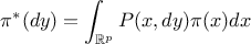
The Markov chain Monte Carlo approach (MCMC) approach works as follows: the invariant distribution is assumed
known, since it is the distribution from which we wish to sample, while the transition kernel is unknown and to be
determined. This might seem to be "the proverbial needle in a haystack" but the idea is to be able to express the target
density using a transition probability kernel  (describing the move from to
  ) as
) as

where  and 0 otherwise, while
 is the probability that the chain remains at its current location. If the transition part of this
function,
is the probability that the chain remains at its current location. If the transition part of this
function,  ,
satisfies the reversibility condition (also called time reversibility,
detailed balance, microscopic reversibility...)
,
satisfies the reversibility condition (also called time reversibility,
detailed balance, microscopic reversibility...)

then  is the invariant density of
 ![]() [tierney1994markov].
[tierney1994markov].
In the MCMC approach, the candidate-generating density is traditionally denoted
 . If this density
satisfies the reversibility condition in Equation Equation VII.13 for
all and the search would be over, but this is very unlikely.
What's more probable is to find something like
. If this density
satisfies the reversibility condition in Equation Equation VII.13 for
all and the search would be over, but this is very unlikely.
What's more probable is to find something like  that states that moving from to occurs too often (or too rarely).
The proposed way to correct this is to introduce a probability  where this
  is called the probability of a
move that is injected in the reversibility condition to help fulfil it. Without
going into too much detail (see [chib1995understanding] which nicely discusses this), the
probability of move is usually set to
is called the probability of a
move that is injected in the reversibility condition to help fulfil it. Without
going into too much detail (see [chib1995understanding] which nicely discusses this), the
probability of move is usually set to
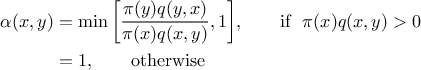
If the chain is currently at a point  , then it generates a value accepted as
  with the probability . If rejected, the chain remains at the current location and
another drawing is performed from there.
with the probability . If rejected, the chain remains at the current location and
another drawing is performed from there.
With this, one can define the off-diagonal density of the MCMC kernel as function  if
if
 and 0 otherwise and
thanks to Equation Equation VII.12, one has the invariant distribution for
[tierney1994markov].
and 0 otherwise and
thanks to Equation Equation VII.12, one has the invariant distribution for
[tierney1994markov].
Warning
Two important things to notice herethe obtained sample is obviously not independent as the (k+1)-th location is taken out from the k-th one. It might thus be useful to thin the obtained sample to ensure that the samples are less correlated (or ideally uncorrelated) with one another thanks to the lag hyperparameter.
the very first drawn locations are usually rejected as part of the burn-in (also called warm-up) process. As discussed above, the algorithm needs a certain number of iterations to converge through the invariant distribution.
The idea here is to choose a family of candidate-generating densities that follow  where
where  is a multivariate density
[muller1991generic], a classical choice being
is a multivariate density
[muller1991generic], a classical choice being  typically chosen as a multivariate normal density. The
candidate is indeed drawn as current value plus a noise, hence the name "random walk".
typically chosen as a multivariate normal density. The
candidate is indeed drawn as current value plus a noise, hence the name "random walk".
Once the newly selected configuration-candidate is chosen, let's call it  , a comparison is made with the latest retained
configuration, denoted
, a comparison is made with the latest retained
configuration, denoted  , through the likelihood ratio, which allows to get rid of any constant factors and should look
like this once transformed to its log form:
, through the likelihood ratio, which allows to get rid of any constant factors and should look
like this once transformed to its log form:

This result is then compared to the logarithm of a random uniform drawing between 0 and 1 to decide whether one should keep this configuration (as is usually done in Monte Carlo approaches, see [chib1995understanding]).
There are a few more properties for this kind of algorithm such as the acceptation ratio, that might be tuned or used as validity check according to the dimension of our parameter space for instance [gelman1996efficient,roberts1997weak] or the lag definition, sometimes used to thin the resulting sample (whose use is not always recommended as discussed in [link2012thinning]). These subjects being very close to the implementation choices, they are not discussed here.
Convergence is often difficult to diagnose in practice. To increase confidence in the results, it is advisable to initialize several chains in Markov Chain Monte Carlo (MCMC). This approach helps assess convergence and improves the reliability of the results. Since MCMC methods sample from a probability distribution by simulating a chain of dependent draws, a single chain might get stuck in a local mode or fail to explore the distribution fully. Running multiple chains from different starting points allows us to check whether they converge to the same target distribution, thereby increasing confidence that the sampling has stabilized. Additionally, comparing chains provides diagnostics for mixing and convergence, making the inference more robust.
As explained before, the Metropolis-Hastings (MH) algorithm proposes updates for the entire parameter vector at once, drawing candidates from a proposal distribution in the full parameter space. This can be efficient when the proposal is well-tuned and captures correlations between parameters, but in high dimensions it is often difficult to design such a proposal, and acceptance rates may become very low.
In contrast, Component-wise Metropolis-Hastings (CMH), also known as the Metropolis-within-Gibbs (MwG) method [tierney1994markov], updates one parameter (or a block of parameters) at a time (selected sequentially or randomly) while keeping the others fixed. This usually leads to higher acceptance rates and easier tuning, especially when parameters are weakly correlated. However, CMH may converge more slowly if strong correlations exist between components, since updates proceed dimension by dimension.
In practice, MH is preferred when a good joint proposal distribution is available or when parameters are highly correlated, while CMH is often advantageous in high-dimensional problems where simpler, one-dimensional proposals are easier to construct and tune.
Assessing convergence is a crucial step when applying MCMC methods, as a lack of convergence can compromise the validity of the inference. In practice, several complementary techniques are used:
a burn-in period is typically discarded to remove the influence of the arbitrary starting point before the chain reaches stationarity;
thinning the chain by keeping only every k-th sample (lag) can reduce autocorrelation between draws;
visual inspection of trace plots is also a simple but powerful way to verify whether the chains have mixed well and stabilized;
monitoring the acceptance ratio provides further information about the efficiency of the algorithm: values that are too high may indicate inefficient exploration, while values that are too low suggest poor mixing.
Beyond these practical checks, formal diagnostics are often employed. The Effective Sample Size (ESS) quantifies the number of effectively independent samples, accounting for autocorrelation [geyer1992]:
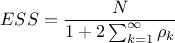
where  is the total number of draws and
  the autocorrelation at lag
  .
In practice, the sum over is
truncated once the autocorrelation becomes small enough, often smaller than 0.05. A larger ESS indicates more
efficient sampling.
.
In practice, the sum over is
truncated once the autocorrelation becomes small enough, often smaller than 0.05. A larger ESS indicates more
efficient sampling.
The Gelman-Rubin statistic  compares within-chain and between-chain variances across multiple chains [gelman1992]:
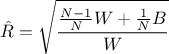
with  the within-chain variance and
  the between-chain variance for
  chains of length .
Values of close to 1
suggest that the chains have converged to the same target distribution.
chains of length .
Values of close to 1
suggest that the chains have converged to the same target distribution.
Together, these diagnostics and techniques provide complementary evidence that the MCMC algorithm has converged and that its samples can be reliably used for inference.
| |  | |
| VII.4. Approximate Bayesian Computation techniques (ABC) |  | VII.6. CIRCE method |