

Documentation
/ Manuel utilisateur en C++
: 
II.2. The TAttribute class | ||
|---|---|---|
 | Chapter II. The DataServer module |  |
The TAttribute class (as its inherited classes, some of which are discussed here as well), is also a crucial part of any
analysis performed through Uranie. It describes any variable (input, output, or internal variable such as iterator)
that are passed to the other modules. It does not really contain the data, but it has the statistical information (in
case methods such as computeStatistic or computeQuantile have been
called, see Section II.4)
Unlike previous Uranie-version where all attribute were double-precision float values, the implementation done from
v3.10.0 allows to handle two other types of attribute: string and vector. There are several ways to define the new
attribute nature, following the chosen construction process, but all these methods will affect the enumerator
URANIE::DataServer::EType whose value can be:
kDefault: the default one which is equal tokRealkString: in the case of text input (assuming that this text is no split into more than one word, unless extra-cautions are taken)kVector: for vectors of double-precision values. Even though the number of elements within this vector can change from one pattern to the other, many useful methods discussed in the following sections and chapters will required (in order to make sense) to have a constant number of elements (at least for a sub-selection of patterns). This is particularly true for all mathematical methods and sensitivity analysis. The code should complain if this requirement is needed and not fulfilled.
This new implementation is bringing changes in the way some information are handled, as for the attribute is concerned, but all the resulting modification have been checked to be backward compatible. Default settings are made assuming that attributes are double-precision ones, unless specified otherwise (to be sure that all previous script will work). The corresponding modifications are discussed throughout this documentation.
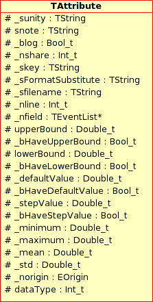
We will present in this section the list of information contained in a TAttribute of Uranie.
- Name: Variable name
- It should be a short name as this information is needed to use this variable (mathematical expressions, graphics, scan, ...).
- Title: Variable title.
- This information is only needed for graphical display.
- Unit: Variable units.
- This information is only needed for graphical display.
- Note: Variable note.
- description of the variable, this is not currently used.
- Min, Max, Mean and Std: Minimum, maximum, averaged and standard deviation values.
- These information are now vectors and their usage is discussed in Section II.4.3
- vquantile: Vector of map containing value of the quantile computed using the key in argument.
- These information are now stored in the attribute itself their usage is discussed in Section II.4.4
- defaultValue: Default value.
- This default value will be considered either by the code launcher or during a parameter optimisation. In the case of a code launcher, this means either that the code failed to proceed or that the code did not return the value.
At this level, there is no notion of random variable. Attributes are variables with a name, a label, a unit, a variation domain (bounded or belonging to R). Despite the large amount of possible combinations to instantiate a variable (name, name+label, name+boundary, name+label+boundary), only a small number of constructors are implemented. Some methods like setTitle, setFileKey, setUnity allow to precise the missing information.
The four constructors currently implemented are the following:
Name: since this constructor only knows the name of the variable, the 3 piece of information title, label and key are strictly identical. This variable is not bounded. An example of use, already seen before, is:
TAttribute *px = new TAttribute("x");A random variable "x" ( where px denotes a pointer to x) exists and it has its label also equal to x. Thus, if this variable is visualised on a graph, the default label will also be its title i.e "x".
Name + title: constructor defined from the name and the title of the variable
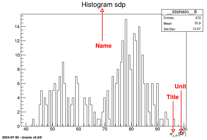
TAttribute *psdp = new TAttribute("sdp", "#sigma_{#Delta P}");
psdp->setUnity("M^{2}");
A pointer psdp to a variable "sdp" is available with title being #sigma_{#Delta P}. The command setUnity() precises the unit. In this case, by default, the field key is identical to the field name. We will use the ability given by ROOT to write LaTeX expressions in graphics to improve graphics rendering without weighing down the manipulation of variables: as a matter of fact, we can plot the histogram of the variable sdp by:
tdsGeyser->addAttribute("newx2","x2","#sigma_{#Delta P}","M^{2}");
tdsGeyser->draw("newx2");
The result of this piece of code is shown in Figure II.3.
Name + variation boundary: constructor defined by the name of the variable and the lower and upper boundaries. The two other pieces of information, label and key remain equal to the title. An example of use is
TAttribute *x = new TAttribute("x", -2.0, 4.0);Name + EType: constructor defined by the name of the variable and nature of the corresponding attribute . An example of use is
TAttribute *xvec = new TAttribute("x", URANIE::DataServer::TAttribute::kVector);
Setter methods allow to fill the other fields (title, key, etc ) generally by calling set and the name of the information to be modified (a restricted list of available methods
being given below). For instance, the plot "x2:x1" of TDataServer data tdsGeyser (whose data file
geyser.dat can be found in the Uranie-macros folder) can be considered again and we can
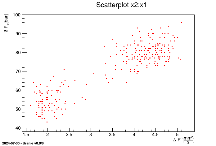
replace the fields title and unit with new values by using LaTeX instructions. For instance, let us consider once again the graph of TDataServer data
tdsGeyser:
TAttribute *px1 = tdsGeyser->getAttribute("x1");
px1->setTitle("#Delta P^{#sigma}"); // Change the title
px1->setUnity("#frac{mm^{2}}{s}"); // Change the unit
tdsGeyser->Draw("x2:x1"); // Draw the plot
The first line consists in retrieving the attribute pointer x1, while the others are self
explanatory. This results in a new graph (scatterplot) of x2 versus x1 for the
TDataServer constructed from the geyser file with updated field title and unit values, shown in Figure II.4.
Figure II.4. Scatterplot x2 versus x1 for the geyser data with modification of fields title and unit.
Most of the information can be modified by "setter" methods. Here is a short list of the most relevant one starting with simple and already discussed attribute properties:
setTitle(TString str): assigns the character string str passed as argument to the field title;
setUnity(TString str): assigns the character string str passed as argument to the field unity;
setNote(TString str): assigns the character string str passed as argument to the field note;
setUpperBound/setLowerBound/setDefaultValue(double val): assigns or changes (if it already existed) respectively the upper, lower or default value for this attribute.
setDataType(EType thetype or TString str): changes the nature of the attribute given the enumerator value or a character chain (case insensitive). In the latter case, the enumerator is set to:
kReal: str= "double" or "real" or "d";
kString: str= "string" or "s"
kVector: str= "vector" or "v"
Given the new nature of attributes (meaning vectors and strings) a more generic method has been created to put default values to all type. The generic methods takes only one argument, a string containing values whatever the type. In cas of doubt, dedicated methods have also been created, with dedicated prototypes:
kReal: both
setDefault(TString value)andBool_t setDefaultValue(Double_t val)can be used as shown belowTAttribute *real = new TAttribute("real"); double real_value=1.23456789; real->setDefaultValue(real_value); // Default with double value real->setDefault("1.23456789"); // Default with generic methodkVector: both
setDefault(TString value)andsetDefaultVectorvector<double> &vec)can be used as shown belowTAttribute *vector = new TAttribute("vector",TAttribute::kVector); std::vector<double> v_value={1.2,2.3,3.4}; vector->setDefaultVector(v_value); // Default with double value vector->setDefault("1.2,2.3,3.4"); // Default with generic methodkString: both
setDefault(TString value)andsetDefaultString(TString val)can be used as shown belowTAttribute *string = new TAttribute("string",TAttribute::kString); TString str_value="chocolat"; string->setDefaultString(str_value); // Default with double value string->setDefault(str_value); // Default with generic method
There are also important setters, used to connect attributes to ASCII files. Most of the time, ASCII files are indeed used to communicate with an external code and Uranie must know in this case where to find the useful information for the corresponding attributes (either to write a new value that would be used as input to perform a calculation or to read the output of another computation). This is more carefully detailed in Section IV.3.1.
setFileKey(TString sfile, TString skey,TString sformatToSubstitute, TAttributeFileKey::EFileType sFileType): allows to specify for an attribute a file sfile, a key linked to this file skey, a writing format of the value of this key in the previous file sformatToSubstitute, and also the type of the file sFileType. This is heavily discussed in Chapter IV.
The following instruction defines a pointer px to an unbounded variable x.
TAttribute *px = new TAttribute("x");The following instruction defines a pointer px to a variable x bounded between 0. and 1.
TAttribute *px = new TAttribute("x", 0., 1.);The following instruction defines a pointer px to a variable x bounded between -2. and 4. with  as label:
TAttribute *px = new TAttribute("x", -2.0, 4.0);
px->setTitle("#Delta P_{e}^{F_{iso}}");
The following instruction defines a pointer px to a variable x that describes string
TAttribute *px = new TAttribute("x", URANIE::DataServer::TAttribute::kString);It is possible to add new attribute in a given TDataServer object that would contain data
using two different methods. The first one rely on the already existing data to create a new variable by simply
writting the equation, which internally is calling a TAttributeFormula object. The following
piece of code shows how to create a third variable from the geyser.dat file, simply as an equation
from the existing variables:
TDataServer *tds = new TDataServer("foo","pouet");
tds->fileDataRead("geyser.dat");
// Adding a new attribute
TAttribute *x3 = new TAttribute("x3","0.5*x2+sin(x1)");
This method can deal with double and vector-based attributes (of course no equation can be estimate when one of the input variable in the formula is a string one, so this method will crash).
Another way recently introduced is to add an attribute from an array of double (or it's equivalent in
python, meaning a numpy.array) by calling the method
addAttributeUsingData. The idea is to be able to add information that would have been
processed by methods aside from the Uranie ones. The signature of the function is the name of the new attribute as
first argumet, the second one is an array of double and the third one is the size of the array. There are two ways,
recommended, that uses object with built-in method that provide the size (to prevent from mis-typing problem between
the array and its size). Obviously, the size of the array must be equal to the number of patterns in the existing
TDataServer object.
Here is an example using the myData.dat, in C++:
TDataServer *tds = new TDataServer("foo","tru");
tds->fileDataRead("myData.dat");
// Defining a vector with 11 elements
vector<double> x2 = {-10,-8,-6,-4,-2,0,2,4,6,8,10};
// Call the method using the address of first element and the size of it
tds->addAttributeUsingData("x2", &x2[0], x2.size());
This method should only be used to create double-based attributes (as the size of the array would be chaotic if it were to be a vector of varying size). Obviously, no string-based attribute can be constructed like this.
Warning
The methodaddAttributeUsingData should only be called either when no data AND no attribute
are stored in the dataserver or when there are data and the new array of double provided has the same size (number of
patterns) as the data already available within the dataserver.
The TStochasticAttribute is the parent class to all attributes which values can be generated by a TSampler (as discussed in Section III.2). All child objects are random variables, following a specific law, that
depends on a small number of parameters.
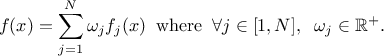
As from version 4.8 of the Uranie platform it is possible to combine different probability law, as a sum of weighted contributions, in order to create a new law. This approach, which is further discussed and illustrated in Section II.2.5.19, leads to a new probability density function that would look like
These distributions can be used to model the behaviour of variables, depending on chosen hypothesis, probability density function being used as a reference more oftenly by physicist, whereas statistical experts will generally use the cumulative distribution function [Appel13].
Table II.1 gathers the list of implemented statistical laws, along with its class name in Uranie and the list of parameters used to define them. For every possible
law, a piece of code is provided to show how to draw a simple PDF, along with a figure
that displays the PDF, CDF and inverse
CDF[1] for different
sets of parameters (the equation of the corresponding PDF is reminded as well on every figure). The inverse CDF is
basically the CDF whose x and y-axis are inverted (it is convenient to keep in mind what it looks like, as it will be
used to produce design-of-experiments, later-on). For all these laws, the parameters can be set at the
constructor (as shown in the previous example block) but, if this has not been done it is possible to change their
value using the setParameters method.
Table II.1. List of Uranie classes representing the probability laws
| Law | Class Uranie | Parameter 1 | Parameter 2 | Parameter 3 | Parameter 4 |
|---|---|---|---|---|---|
| Uniform | TUniformDistribution | Min | Max | ||
| Log-Uniform | TLogUniformDistribution | Min | Max | ||
| Triangular | TTriangularDistribution | Min | Max | Mode | |
| Log-Triangular | TLogTriangularDistribution | Min | Max | Mode | |
| Normal (Gauss) | TNormalDistribution | Mean ( ) ) | Sigma ( ) ) | ||
| Log-Normal | TLogNormalDistribution | Mean ( ) ) | Error factor ( ) ) | Min | |
| Trapezium | TTrapeziumDistribution | Min | Max | Low | Up |
| UniformByParts | TUniformByPartsDistribution | Min | Max | Median | |
| Exponential | TExponentialDistribution | Rate ( ) ) | Min | ||
| Cauchy | TCauchyDistribution | Scale ( ) ) | Median | ||
| GumbelMax | TGumbelMaxDistribution | Mode () | Scale ( ) )
| ||
| Weibull | TWeibullDistribution | Scale () | Shape ( ) ) | Min | |
| Beta | TBetaDistribution | alpha ( ) ) | beta () | Min | Max |
| GenPareto | TGenParetoDistribution | Location () | Scale () | Shape ( ) ) | |
| Gamma | TGammaDistribution | Shape () | Scale () | Location ( ) ) | |
| InvGamma | TInvGammaDistribution | Shape () | Scale () | Location () | |
| Student | TStudentDistribution | DoF () | |||
| GeneralizedNormal | TGeneralizedNormalDistribution | Location () | Scale () | Shape () |
To define a random variable, the corresponding constructor must be used. The arguments of these constructors are first, the name of the variable and second, the parameters of the law. For example:
//Uniform law
TUniformDistribution *pxu = new TUniformDistribution("x1", -1.0 , 1.0);
// Gaussian Law
TNormalDistribution *pxn = new TNormalDistribution("x2", -1.0 , 1.0);
// Gaussian Law
TNormalDistribution *pxn = new TNormalDistribution("x2", -1.0 , 1.0); 
Allocation of a pointer pxu to a random uniform variable x1 in interval [-1.0, 1.0]. | |
Allocation of a pointer pxn to a random normal variable x2 with mean value μ=-1.0 and standard deviation σ=1.0. |
These distributions can be used to model the behaviour of inputs, the choice being generally based on the way the PDF looks like. For every distributions implemented in Uranie examples of PDF, CDF and inverse CDF are show from Figure II.5 until Figure II.28. Here is a brief description of the probability density functions and their parameters.
The Uniform law is defined between a minimum and a maximum, as
Uranie code to simulate an uniform random variable is:
TDataServer *tds = new TDataServer("tdssampler", "Sampler Uranie demo");
tds->addAttribute( new TUniformDistribution("u", -2., 3.));

TSampling *fsamp = new TSampling(tds, "lhs", 300);
fsamp->generateSample(); // Create a representative sample

tds->Draw("u");
Figure II.5 shows the PDF, CDF and inverse CDF generated for a given set of parameters.
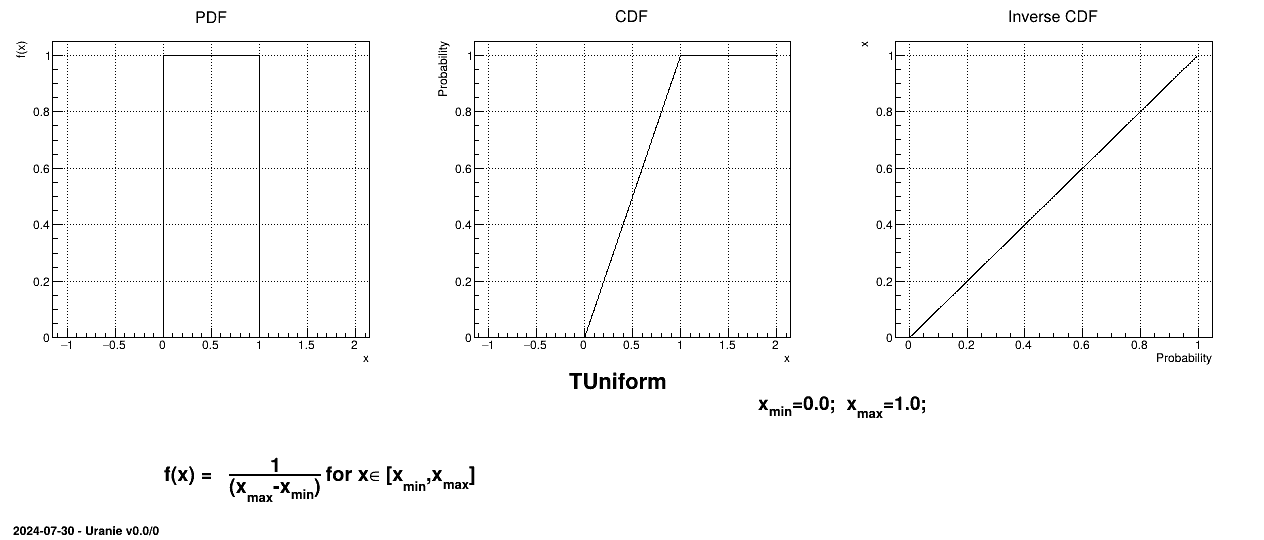
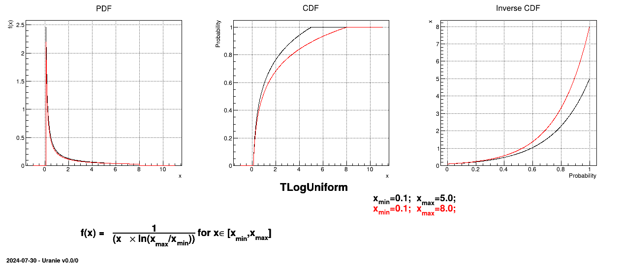
The LogUniform law is well adapted for variations of high amplitudes. If a random variable  follows a LogUniform distribution, the random variable
 follows a Uniform
distribution, so
follows a Uniform
distribution, so
Uranie code to simulate a LogUniform random variable is:
TDataServer *tds = new TDataServer("tdssampler", "Sampler Uranie demo");
tds->addAttribute( new TLogUniformDistribution("lu", .001, 10.));

TSampling *fsamp = new TSampling(tds, "lhs", 300);
fsamp->generateSample(); // Create a representative sample

tds->Draw("lu");
tds->Draw("log(lu)"); // Check that ln(x) follows a uniform law
Figure II.6 shows the PDF, CDF and inverse CDF generated for different sets of parameters.
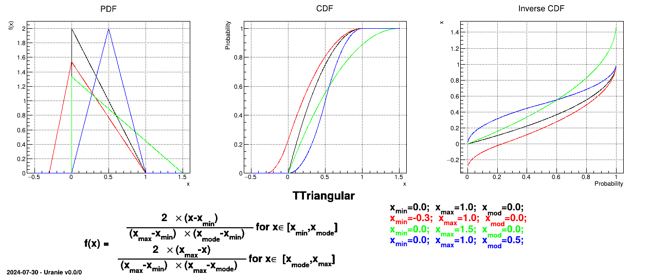
This law describes a triangle with a base between a minimum and a maximum and a highest density at a certain point
 , so
, so

Uranie code to simulate a triangular random variable is:
TDataServer *tds = new TDataServer("tdssampler", "Sampler Uranie demo");
tds->addAttribute( new TTriangularDistribution("t", 5.0, 8., 6.0));

TSampling *fsamp = new TSampling(tds, "lhs", 300);
fsamp->generateSample(); // Create a representative sample

tds->Draw("t");
Figure II.7 shows the PDF, CDF and inverse CDF generated for different sets of parameters.
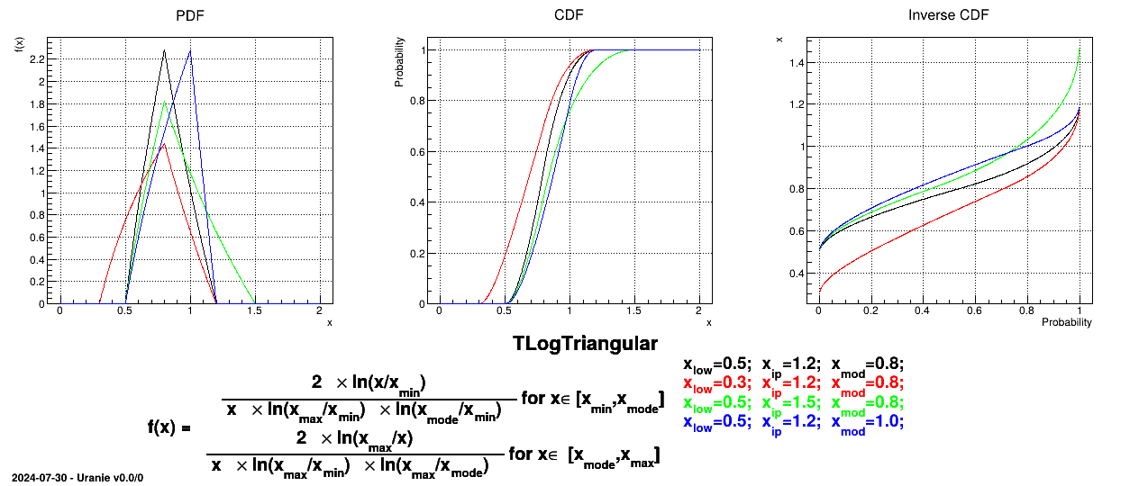
If a random variable follows a
LogTriangular distribution, the random variable follows a Triangular distribution, so

and

Uranie code to simulate a LogTriangular random variable is:
TDataServer *tds = new TDataServer("tdssampler", "Sampler Uranie demo");
tds->addAttribute( new TLogTriangularDistribution("lt", .001, 10., 2.5));

TSampling *fsamp = new TSampling(tds, "lhs", 300);
fsamp->generateSample(); // Create a representative sample

tds->Draw("lt");
tds->Draw("log(lt)"); // Check that ln(lt) follows a triangular law
Figure II.8 shows the PDF, CDF and inverse CDF generated for different sets of parameters.
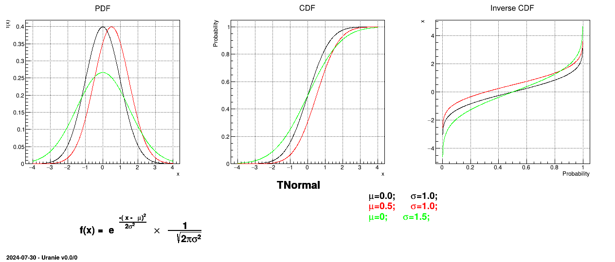
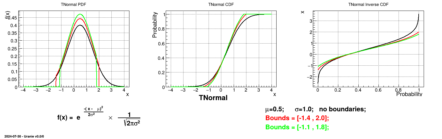
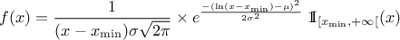
A normal law is defined with a mean and a standard deviation
, as
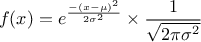
Uranie code to simulate a normal random variable is:
TDataServer *tds = new TDataServer("tdssampler", "Sampler Uranie demo");
tds->addAttribute( new TNormalDistribution("n", 0.0, 1.0));

TSampling *fsamp = new TSampling(tds, "lhs", 300);
fsamp->generateSample(); // Create a representative sample

tds->Draw("n");
Figure II.9 shows the PDF, CDF and inverse CDF generated for different sets of parameters.
Is it also possible to set boundaries to the infinite span of this distribution to create a truncated normal law. This can be done by calling the following method:
tds->getAttribute("n")->setBounds(-1.4,2.0); //truncate the lawThe resulting PDF, CDF and inverse CDF, with and without truncation, can be seen, in this case, in Figure II.10 for a given set of parameters and various boundaries.
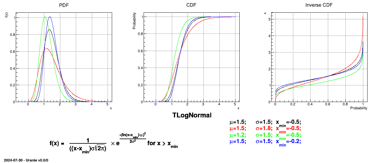
If a random variable follows a
LogNormal distribution, the random variable follows a Normal distribution (whose parameters are and ), so
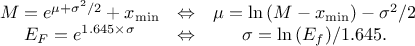
In Uranie, it is parametrised by default using M, the mean of the distribution, , the Error factor that represents the ration of the
95% quantile and the median (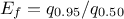 ) and the minimum
  . One can go from one parametrisation to the other following those
simple relations
. One can go from one parametrisation to the other following those
simple relations
Uranie code to simulate a LogNormal random variable is:
TDataServer *tds = new TDataServer("tdssampler", "Sampler Uranie demo");
// using M, Ef and xmin
tds->addAttribute( new TLogNormalDistribution("ln", 1.2, 1.5, -0.5));
// to use ln(x) properties
// double mu = 0.5, sigma=1.; tds->setUnderlyingNormalParameters(mu,sigma);

TSampling *fsamp = new TSampling(tds, "lhs", 300);
fsamp->generateSample(); // Create a representative sample

tds->Draw("ln");
tds->Draw("log(ln)"); // Check that ln(ln) follows a normal law
Figure II.11 shows the PDF, CDF and inverse CDF generated for different sets of parameters.
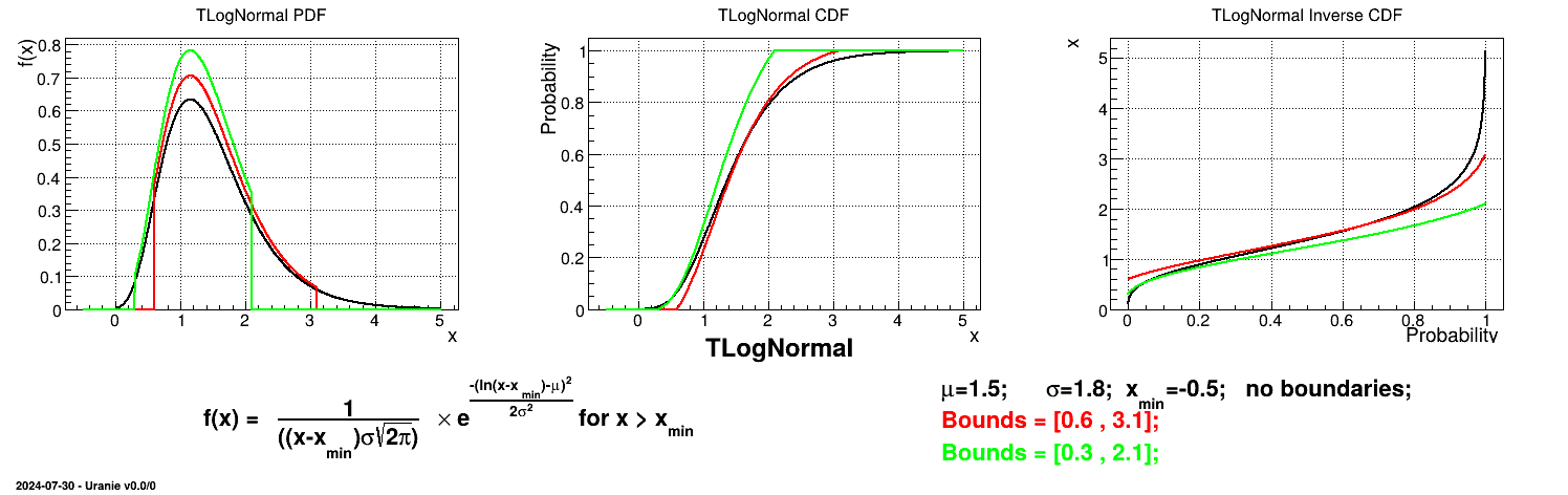
Is it also possible to set boundaries to the infinite span of this distribution to create a truncated normal law. This can be done by calling the following method:
tds->getAttribute("ln")->setBounds(0.6,3.1); //truncate the lawThe resulting PDF, CDF and inverse CDF, with and without truncation, can be seen, in this case, in Figure II.12 for a given set of parameters and various boundaries.
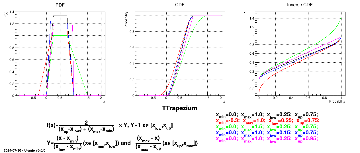
This law describes a trapezium whose large base is defined between a minimum and a maximum and its small base lies between a low and an up value, as
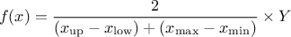
where 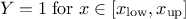 ,
, 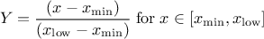 and
and 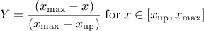 .
.
Uranie code to simulate a Trapezium random variable is:
TDataServer *tds = new TDataServer("tdssampler", "Sampler Uranie demo");
tds->addAttribute( new TTrapeziumDistribution("tr", 0.0, 1.0, 0.25, 0.75) );

TSampling *fsamp = new TSampling(tds, "lhs", 300);
fsamp->generateSample(); // Create a representative sample

tds->Draw("tr");
Figure II.13 shows the PDF, CDF and inverse CDF generated for different sets of parameters.
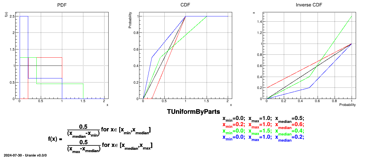
The UniformByParts law is defined between a minimum and a median and between the median and a maximum, as

Uranie code to simulate a UniformByParts random variable is:
TDataServer *tds = new TDataServer("tdssampler", "Sampler Uranie demo");
tds->addAttribute( new TUniformByPartsDistribution("ubp", 0.0, 1.0, 0.5) );

TSampling *fsamp = new TSampling(tds, "lhs", 300);
fsamp->generateSample(); // Create a representative sample

tds->Draw("ubp");
Figure II.14 shows the PDF, CDF and inverse CDF generated for different sets of parameters.
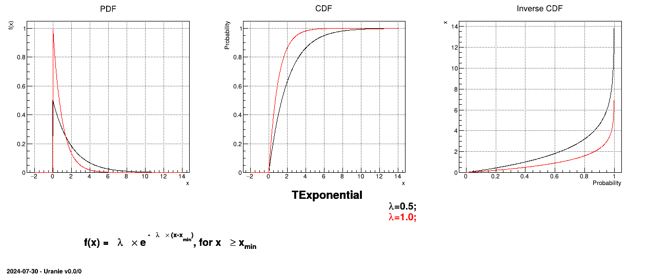
This law describes an exponential with a rate parameter and a minimum , as

The rate parameter should be greater than 0.0001.
Uranie code to simulate an Exponential random variable is:
TDataServer *tds = new TDataServer("tdssampler", "Sampler Uranie demo");
tds->addAttribute( new TExponentialDistribution("exp", 0.5));

TSampling *fsamp = new TSampling(tds, "lhs", 300);
fsamp->generateSample(); // Create a representative sample

tds->Draw("exp");
Figure II.15 shows the PDF, CDF and inverse CDF generated for different sets of parameters.
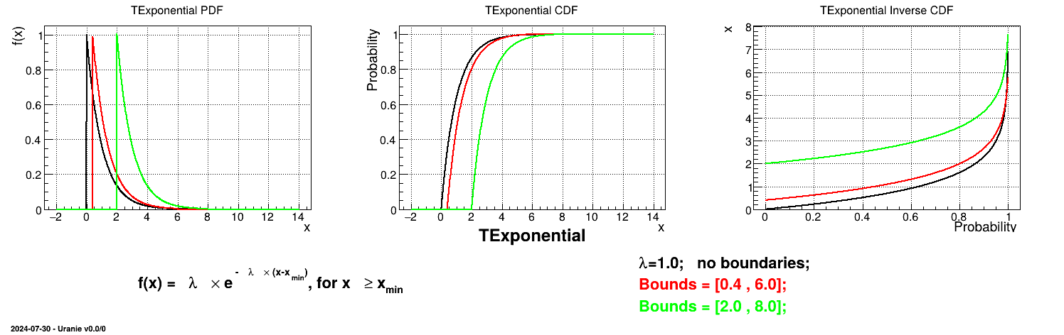
Is it also possible to set boundaries to the infinite span of this distribution to create a truncated Exponential law. This can be done by calling the following method:
tds->getAttribute("exp")->setBounds(0.4,6.0); //truncate the lawThe resulting PDF, CDF and inverse CDF, with and without truncation, can be seen, in this case, in Figure II.16 for a given set of parameters and various boundaries.
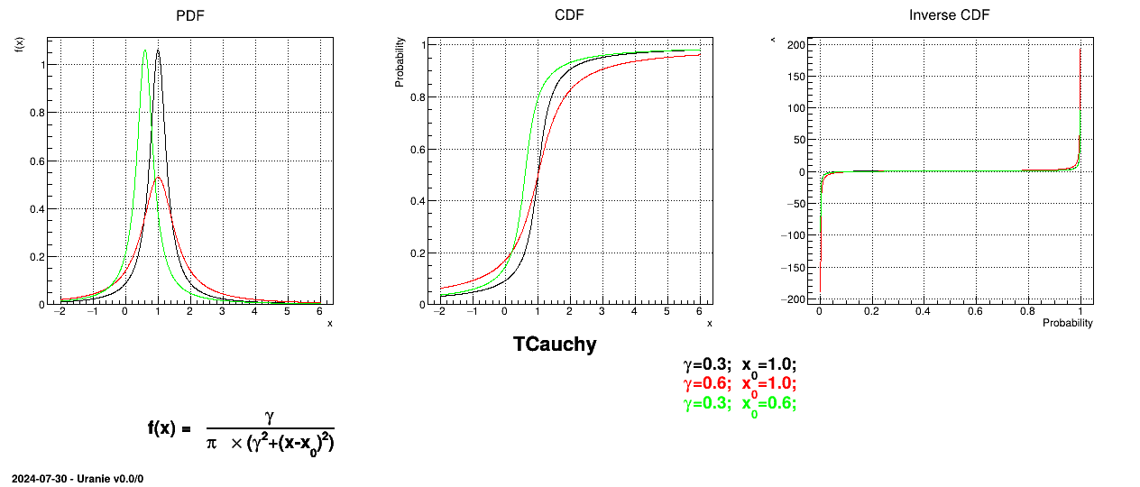
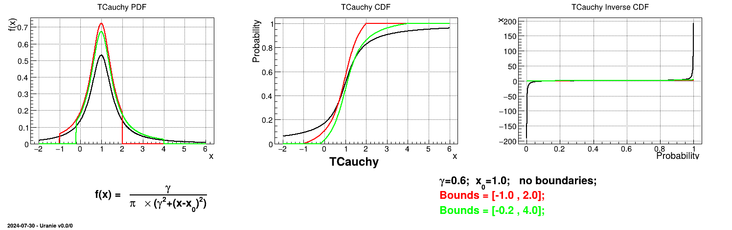
This law describes a Cauchy-Lorentz distribution with a location parameter  and a scale parameter , as
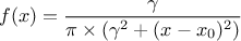
The parameter should be greater than 0.0001.
Uranie code to simulate a Cauchy random variable is:
TDataServer *tds = new TDataServer("tdssampler", "Sampler Uranie demo");
tds->addAttribute( new TCauchyDistribution("cau", 0.3, 1.0));

TSampling *fsamp = new TSampling(tds, "lhs", 300);
fsamp->generateSample(); // Create a representative sample

tds->Draw("cau");
Figure II.17 shows the PDF, CDF and inverse CDF generated for different sets of parameters.
Is it also possible to set boundaries to the infinite span of this distribution to create a truncated Cauchy law. This can be done by calling the following method:
tds->getAttribute("cau")->setBounds(-1.0,2.0); //truncate the lawThe resulting PDF, CDF and inverse CDF, with and without truncation, can be seen, in this case, in Figure II.18 for a given set of parameters and various boundaries.
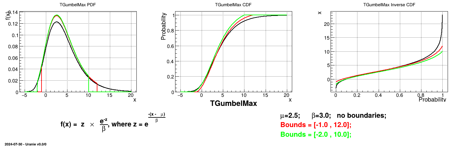
This law describes a Gumbel max distribution depending on the mode and the scale , as
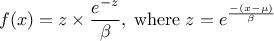
The scale should be greater than 0.000001 times
Uranie code to simulate a GumbelMax random variable is:
TDataServer *tds = new TDataServer("tdssampler", "Sampler Uranie demo");
tds->addAttribute( new TGumbelMaxDistribution("gm", 0.5, 2.0));

TSampling *fsamp = new TSampling(tds, "lhs", 300);
fsamp->generateSample(); // Create a representative sample

tds->Draw("gm");
Figure II.19 shows the PDF, CDF and inverse CDF generated for different sets of parameters.
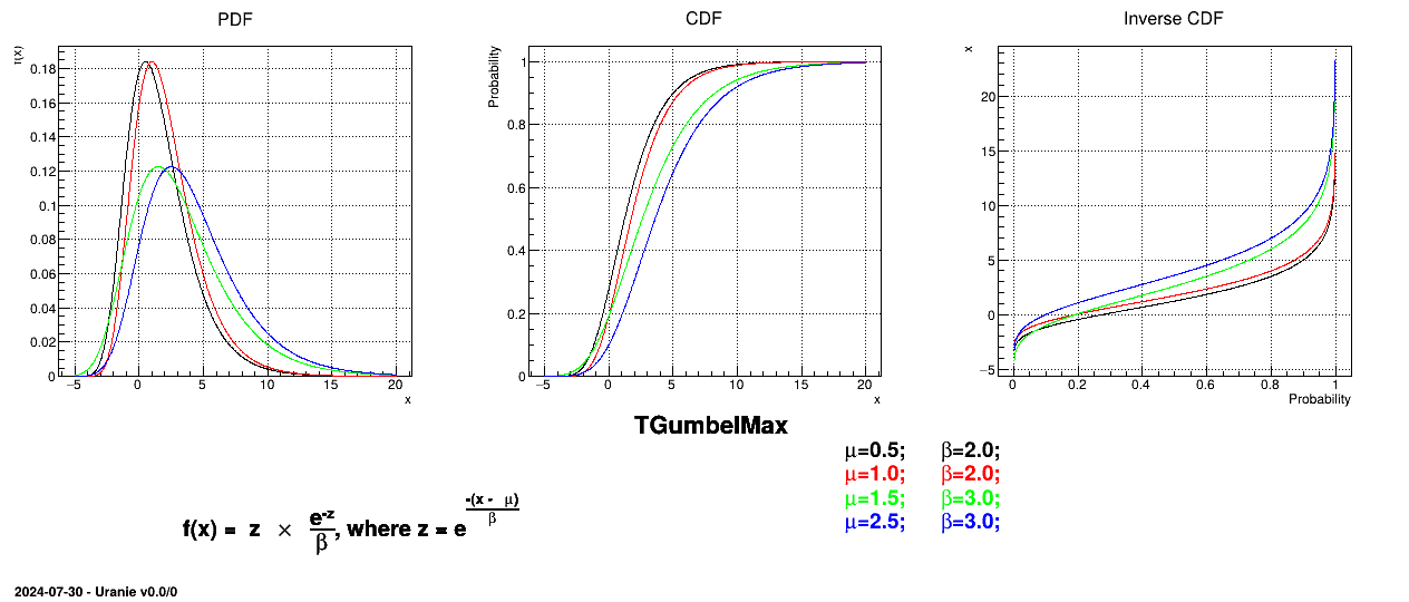
Is it also possible to set boundaries to the infinite span of this distribution to create a truncated GumbelMax law. This can be done by calling the following method:
tds->getAttribute("gm")->setBounds(-1.0,12.0); //truncate the lawThe resulting PDF, CDF and inverse CDF, with and without truncation, can be seen, in this case, in Figure II.20 for a given set of parameters and various boundaries.
This law describes a weibull distribution depending on the location , the scale and the shape q , as
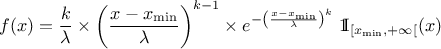
Both and should be greater than 0.0001.
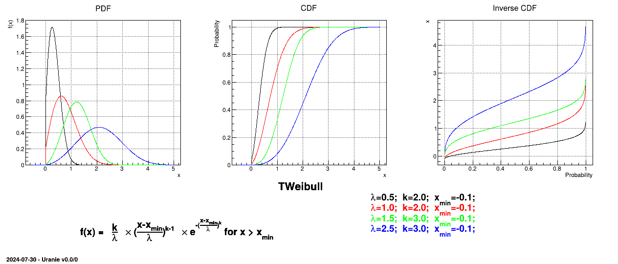
Uranie code to simulate a Weibull random variable is:
TDataServer *tds = new TDataServer("tdssampler", "Sampler Uranie demo");
tds->addAttribute( new TWeibullDistribution("wei", 0.5, 2.0, -0.01) );

TSampling *fsamp = new TSampling(tds, "lhs", 300);
fsamp->generateSample(); // Create a representative sample

tds->Draw("wei");
Figure II.21 shows the PDF, CDF and inverse CDF generated for different sets of parameters.
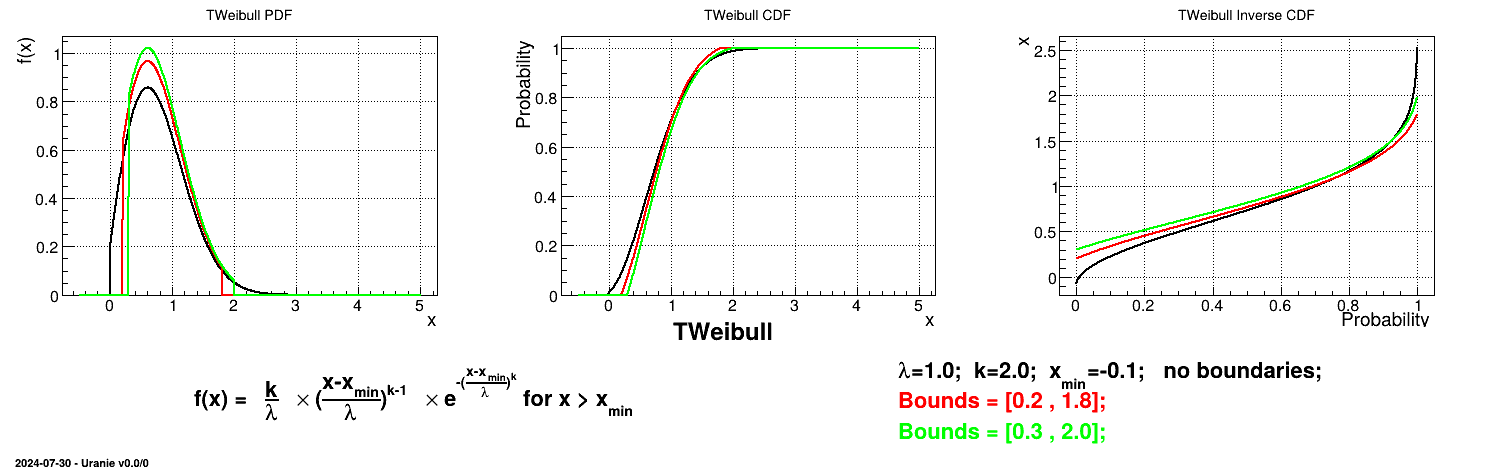
Is it also possible to set boundaries to the infinite span of this distribution to create a truncated Weibull law. This can be done by calling the following method:
tds->getAttribute("wei")->setBounds(0.2,1.8); //truncate the lawThe resulting PDF, CDF and inverse CDF, with and without truncation, can be seen, in this case, in Figure II.22 for a given set of parameters and various boundaries.
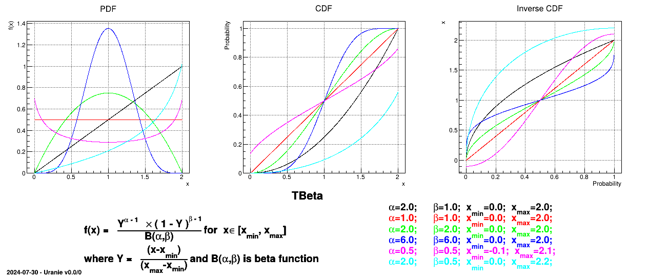
Defined between a minimum and a maximum, it depends on two parameters and , as
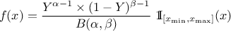
where  and
and  is the
beta function. In the current implementation, both and must be greater than 0.0001.
is the
beta function. In the current implementation, both and must be greater than 0.0001.
Uranie code to simulate a Beta random variable is:
TDataServer *tds = new TDataServer("tdssampler", "Sampler Uranie demo");
tds->addAttribute( new TBetaDistribution("bet", 6.0, 6.0, 0.0, 2.0) );

TSampling *fsamp = new TSampling(tds, "lhs", 300);
fsamp->generateSample(); // Create a representative sample

tds->Draw("bet");
Figure II.23 shows the PDF, CDF and inverse CDF generated for different sets of parameters.
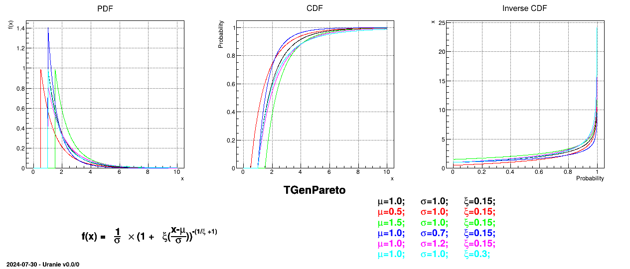
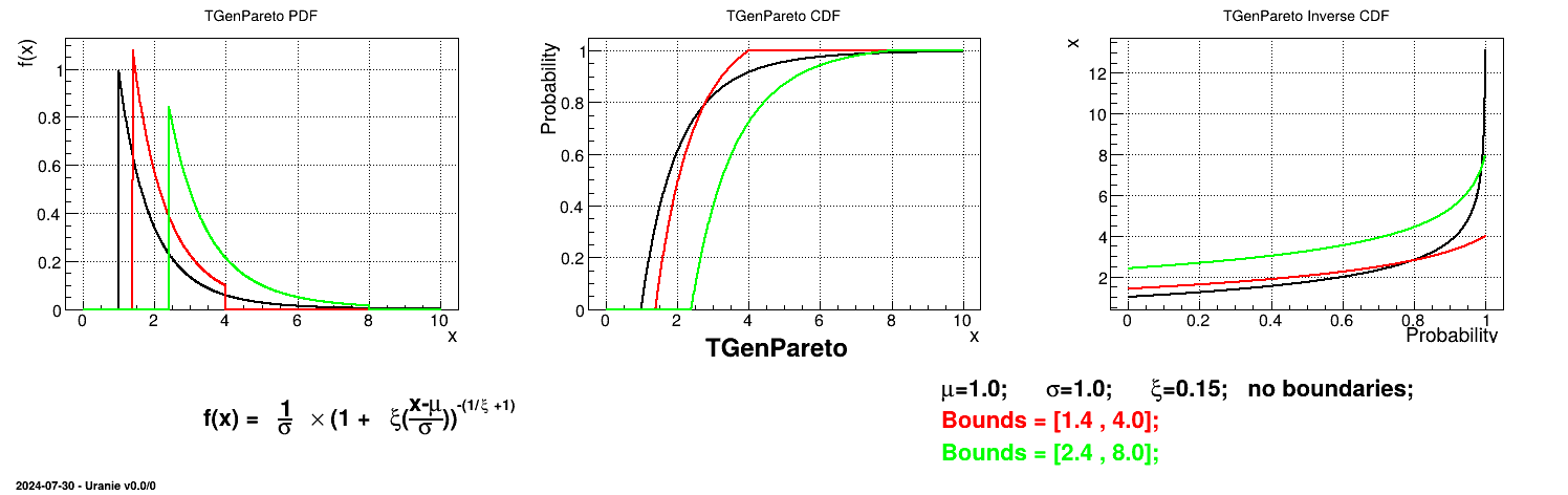
This law describes a generalised Pareto distribution depending on the location , the scale and a shape , as
In this formula, should be greater than 0.
Uranie code to simulate a GenPareto random variable is:
TDataServer *tds = new TDataServer("tdssampler", "Sampler Uranie demo");
tds->addAttribute( new TGenParetoDistribution("gpa", 1.0, 1.0, 0.3));

TSampling *fsamp = new TSampling(tds, "lhs", 300);
fsamp->generateSample(); // Create a representative sample

tds->Draw("gpa");
Figure II.24 shows the PDF, CDF and inverse CDF generated for different sets of parameters.
Is it also possible to set boundaries to the infinite span of this distribution to create a truncated GenPareto law. This can be done by calling the following method:
tds->getAttribute("gpa")->setBounds(1.4,4.0); //truncate the lawThe resulting PDF, CDF and inverse CDF, with and without truncation, can be seen, in this case, in Figure II.25 for a given set of parameters and various boundaries.
The Gamma distribution is a two-parameter family of continuous probability distributions. It depends on a shape
parameter and a scale
parameter . The function
is usually defined for greater
than 0, but the distribution can be shifted thanks to the third parameter called location () which should be positive. This
parametrisation is more common in Bayesian statistics, where the gamma distribution is used as a conjugate prior
distribution for various types of laws:
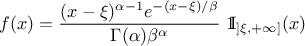
Uranie code to simulate a Gamma random variable is:
TDataServer *tds = new TDataServer("tdssampler", "Sampler Uranie demo");
tds->addAttribute( new TGammaDistribution("gam", 1.0, 2.0, 0.0)) ;

TSampling *fsamp = new TSampling(tds, "lhs", 300);
fsamp->generateSample(); // Create a representative sample

tds->Draw("gam");
Figure II.26 shows the PDF, CDF and inverse CDF generated for different sets of parameters.
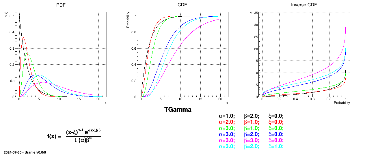
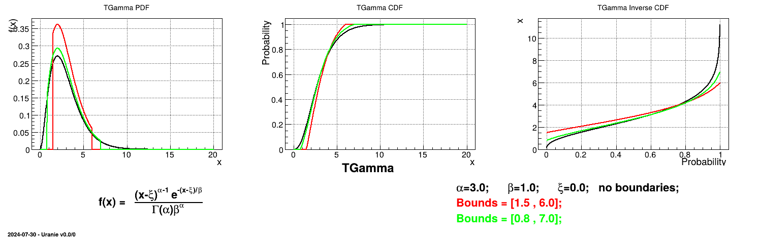
Is it also possible to set boundaries to the infinite span of this distribution to create a truncated Gamma law. This can be done by calling the following method:
tds->getAttribute("gam")->setBounds(0.1,1.6); //truncate the lawThe resulting PDF, CDF and inverse CDF, with and without truncation, can be seen, in this case, in Figure II.27 for a given set of parameters and various boundaries.
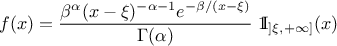
The inverse-Gamma distribution is a two-parameter family of continuous probability distributions. It depends on a shape
parameter and a scale
parameter . The function
is usually defined for greater
than 0, but the distribution can be shifted thanks to the third parameter called location () which should be positive.
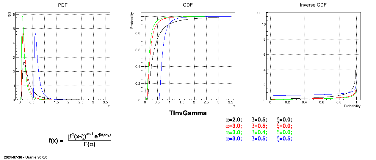
Uranie code to simulate a inverse-Gamma random variable is:
TDataServer *tds = new TDataServer("tdssampler", "Sampler Uranie demo");
tds->addAttribute( new TInvGammaDistribution("ing", 2.0, 0.5, 0.0));

TSampling *fsamp = new TSampling(tds, "lhs", 300);
fsamp->generateSample(); // Create a representative sample

tds->Draw("ing");
Figure II.28 shows the PDF, CDF and inverse CDF generated for different sets of parameters.
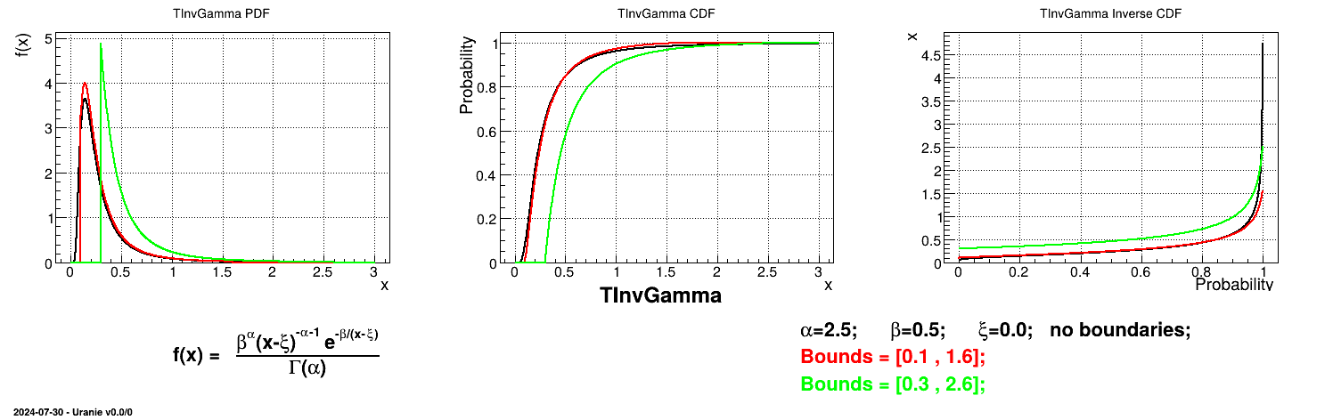
Is it also possible to set boundaries to the infinite span of this distribution to create a truncated InvGamma law. This can be done by calling the following method:
tds->getAttribute("ing")->setBounds(-3.0,8.0); //truncate the lawThe resulting PDF, CDF and inverse CDF, with and without truncation, can be seen, in this case, in Figure II.29 for a given set of parameters and various boundaries.
Warning
This distribution is available only if the ROOT "mathmore" feature has been installed when your ROOT version was brought (you can check this by running
root-config
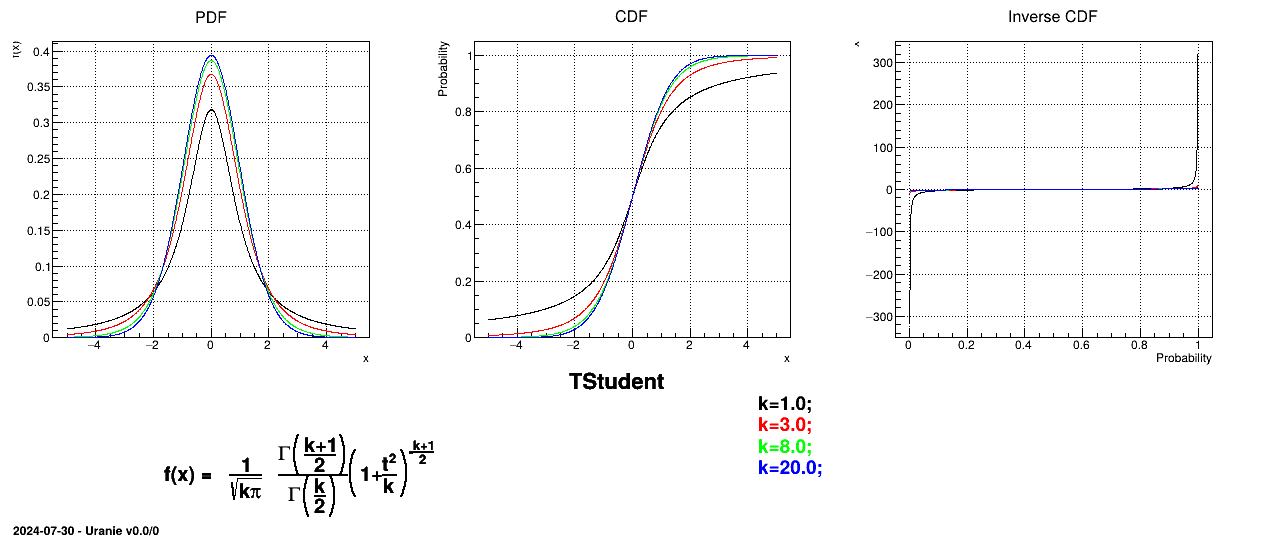
--has-mathmore. If not found, this law cannot be used. The Student law is simply defined with a single parameter: the degree-of-freedom (DoF). The probability density function is then set as
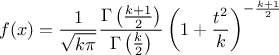
where  is the Euler's gamma function.
Uranie code to simulate an student random variable is:
TDataServer *tds = new TDataServer("tdssampler", "Sampler Uranie demo");
tds->addAttribute( new TStudentDistribution("stu", 5));

TSampling *fsamp = new TSampling(tds, "lhs", 300);
fsamp->generateSample(); // Create a representative sample

tds->Draw("stu");
Figure II.30 shows the PDF, CDF and inverse CDF generated for different sets of parameters.
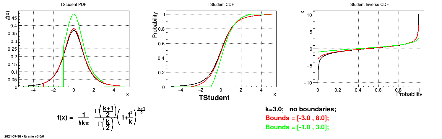
Is it also possible to set boundaries to the infinite span of this distribution to create a truncated Student law. This can be done by calling the following method:
tds->getAttribute("stu")->setBounds(-1.4,2.0); //truncate the lawThe resulting PDF, CDF and inverse CDF, with and without truncation, can be seen, in this case, in Figure II.31 for a given set of parameters and various boundaries.
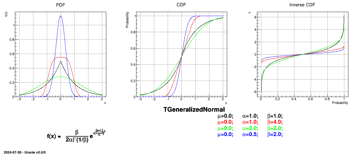
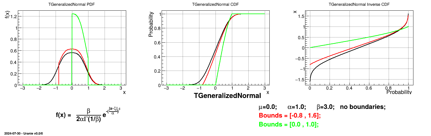
This law describes a generalized normal distribution depending on the location , the scale and the shape q , as
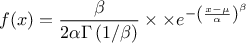
Both
and should be greater than 0.
Uranie code to simulate a generalized normal random variable is:
TDataServer *tds = new TDataServer("tdssampler", "Sampler Uranie demo");
tds->addAttribute( new TGeneralizedNormalDistribution("gennor", 0.0, 1.0, 3.0) );

TSampling *fsamp = new TSampling(tds, "lhs", 300);
fsamp->generateSample(); // Create a representative sample

tds->Draw("gennor");
Figure II.32 shows the PDF, CDF and inverse CDF generated for different sets of parameters.
Is it also possible to set boundaries to the infinite span of this distribution to create a truncated generalized normal law. This can be done by calling the following method:
tds->getAttribute("gennor")->setBounds(-0.8,1.6); //truncate the lawThe resulting PDF, CDF and inverse CDF, with and without truncation, can be seen, in this case, in Figure II.33 for a given set of parameters and various boundaries.
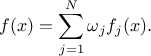
It is possible to imagine a new law, hereafter called composed law, by combining different
pre-existing laws in order to model a wanted behaviour. This law would be defined with  pre-existing laws whose densities are noted
 , along with their relative weights
 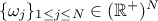 and the resulting density is then written as
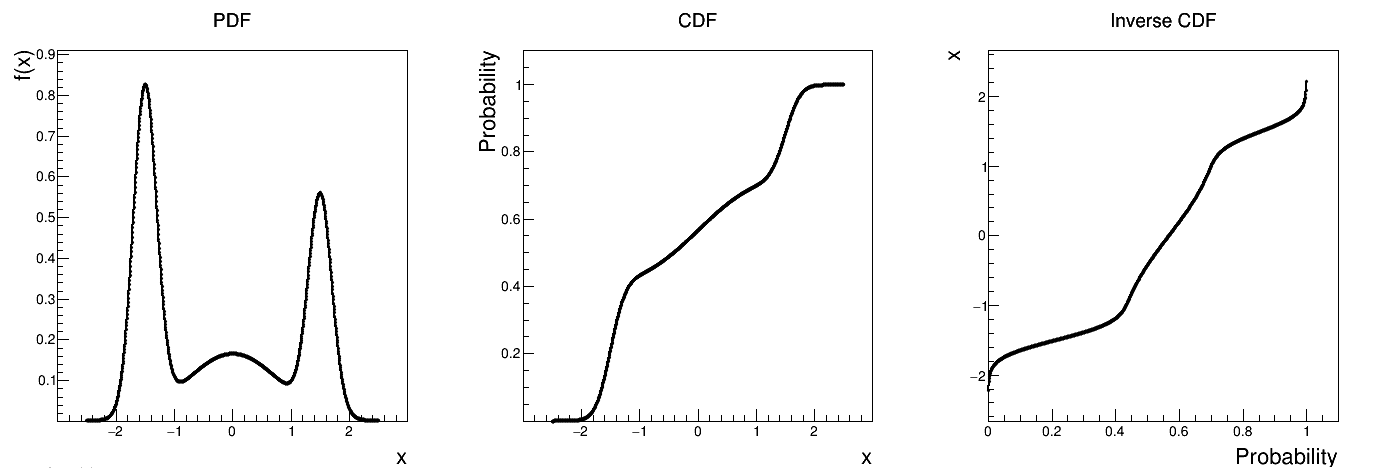
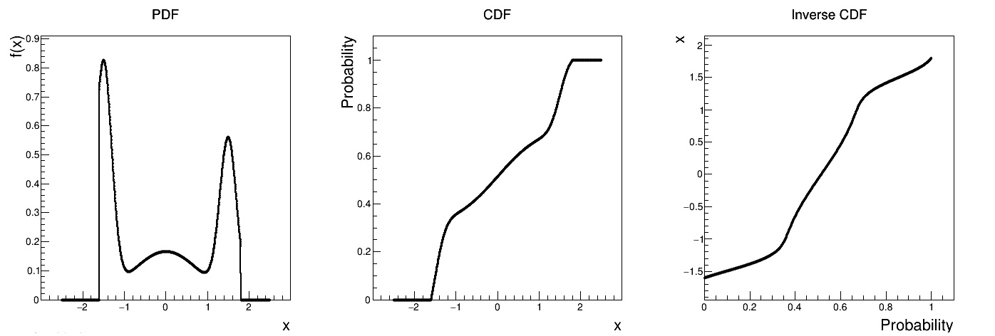
Uranie code to simulate a composition of three normally-distributed laws (with their own statistical properties):
TDataServer *tds = new TDataServer("tdssampler", "Sampler Uranie demo");
TComposedDistribution *comp = new TComposedDistribution("compo");
comp->addDistribution(new TNormalDistribution("n1", -1.5, 0.2), 1.2);
comp->addDistribution(new TNormalDistribution("n2", 0, 0.8), 1.0);
comp->addDistribution(new TNormalDistribution("n3", 1.5, 0.2), 0.8);
tds->addAttribute(comp);

TSampling *fsamp = new TSampling(tds, "lhs", 300);
fsamp->generateSample(); // Create a representative sample

tds->Draw("compo");
Figure II.34 shows the PDF, CDF and inverse CDF generated for different sets of parameters.
Figure II.34. Example of PDF, CDF and inverse CDF for a composed distribution made out of three normal distributions with respective weights.
 |
Is it also possible to set boundaries to the infinite span of this distribution, if it is created from at least one infinite-based law, to create a truncated composed law. This can be done by calling the following method:
tds->getAttribute("compo")->setBounds(-1.6,1.8); //truncate the lawThe resulting PDF, CDF and inverse CDF, with and without truncation, can be seen, in this case, in Figure II.35 for a given set of parameters and various boundaries.
Figure II.35. Example of PDF, CDF and inverse CDF for a truncated composed distribution made out of three normal distributions with respective weights.
 |
The only specific method that is new for the composition is the addDistribution method
whose signature is the following one:
int addDistribution(URANIE::DataServer::TStochasticAttribute *statt, double weight=1.);
The first element is a pointer to a TStochasticAttribute (so any object that is an instance
of a class that derives form it). The second one is the weight (which is 1 by default) and which is the
 constant written in the formula above.
Warning
The theoretical element (mean, standard deviation and mode) can not always be measured for certain stochastic distribution (see the Cauchy's one for instance).- If one wants to add such a distribution in a composed law, a warning exception should pop-up to state that theoretical properties can not be estimated.
- As for the mode, several distributions prevent from having a single-point mode estimation (for instance the Uniform distribution). The mode estimation should then be taken with great care.
| |  | |
| Chapter II. The DataServer module |  | II.3. Data handling |