Documentation / Manuel utilisateur en C++ :

The constructors available for creating an instance of the TLinearBayesian class are those detailed in Section XI.2.3. As a reminder, the available prototypes are:

// Constructor with a runner
TLinearBayesian(TDataServer *tds, TRun *runner, Int_t ns=1, Option_t *option="");
// Constructor with a TCode
TLinearBayesian(TDataServer *tds, TCode *code, Int_t ns=1, Option_t *option="");
// Constructor with a function using Launcher
TLinearBayesian(TDataServer *tds, void (*fcn)(Double_t*,Double_t*), const char *varexpinput, const char *varexpoutput, int ns=1, Option_t *option="");
TLinearBayesian(TDataServer *tds, const char *fcn, const char *varexpinput, const char *varexpoutput, int ns=1, Option_t *option="");
        

Details about these constructors can be found in Section XI.2.3.1, Section XI.2.3.2, and Section XI.2.3.3 respectively for the TRun, TCode, and TLauncherFunction-based constructor. In all cases, the number of samples is set to 1 by default, and modifying it has no effect on the results, since it returns the analytical distributions. This class does not define any specific options.

The final step is to construct the TDistanceLikelihoodFunction, a mandatory step that must always immediately follow the constructor. This can be done via the setLikelihood method (following the prototype presented in Section XI.2.2.1).

void setLikelihood(TDistanceLikelihoodFunction *likelihoodFunc, TDataServer *tdsRef, const char *input, const char *reference, const char *weight="");
          

Once the TLinearBayesian instance is created along with its TDistanceLikelihoodFunction, two methods must be called before performing parameter estimate. These methods are mandatory, as they define the analytical formula used to obtain the Gaussian parameter values of the a posteriori distribution (see [metho]).

The first method (although the order is not important) is setRegressor, whose prototype is

void setRegressor(const char *regressorname);
        

The only argument is regressorname, a string containing the list of regressor names separated by ":". The method then performs two checks: it verifies that the number of regressors matches the number of parameters to be calibrated and it checks that every regressor name provided matches one existing attribute in the reference TDataServer (tdsref). If the observation TDataServer does not contain the regressors (when the input file is loaded) these attributes must be constructed from scratch, either with TAttributeFormula or by using another dedicated assessor (as done in the use-case shown in Section XIV.11.3).

The other method is setObservationCovarianceMatrix whose prototype is

void setObservationCovarianceMatrix(TMatrixD &mat);
        

The only argument here is a TMatrixD whose content is the covariance matrix of the reference observation data. Once again, this method will check two things:

Once these conditions are satisfied, estimate can proceed. One can find an example of how to use these methods in the use-case dedicated subsection (see Section XIV.11.3).

Finally, once the computation is complete there are three different kinds of results, with several ways to interpret and transform them. This section describes some important and specific aspects of these results.

XI.4.3.1. Transformation of the results

The idea is that when you want to consider your model as linear, you may need to slightly transform it to ensure proper linear behaviour and to express and compute the needed regressors. For this particular situation, the use-case described in Section XIV.11.3 will be used. In this case, the flowrate function should be linearised as follows:

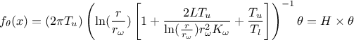
where the regressor can be expressed as 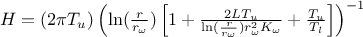. From this, it is clear that we will be calibrating a newly defined parameter . Therefore, at some point, we will need to transform it back into our parameter of interest.

This is the reason why the setParameterTransformationFunction method has been implemented: to transform the estimated parameters given the linear regressor, the observation covariance matrix, and the prior distribution. Since the transformations, if they exist (they are optional), are expected to be carried out using simple operations with constant values, they should affect only the mean vector and not the covariance matrix of the posterior multivariate normal distribution. The prototype of this function is as follows:

void setParameterTransformationFunction(void (*fTransfoParam)(double *in, double *out));
          

Its only argument is a pointer to the transformation function. This function, used to obtain the transformed parameter values, takes two arguments: the input parameters, which are the raw values estimated from the analytical formula detailed in [metho], and the output parameters, which correspond to the desired transformed values. Both arguments are double arrays of length equal to the number of parameters.

The example provided in the use-case Section XIV.11.3 is simple as there is only one parameter to be estimated, which implies that both arguments are one-dimensional double arrays which should look like this:

void transf(double *x, double *res)
{
    res[0] = 1050 - x[0];  // simply H_l = \theta - H_u
}
          

void drawParameters(TString sTitre, const char *variable = "*", Option_t * option = "");
          

void computePredictionVariance(URANIE::DataServer::TDataServer *tdsPred, string outname);