Documentation / Manuel utilisateur en Python :

III.4. QMC method

III.4. QMC method
	Chapter III. The Sampler module

III.4. QMC method

The deterministic samplings can produce design-of-experiments with well defined properties, that can be very useful in specific cases such as:

to cover at best the space of the input variables
to explore the extreme cases
to study combined or non-linearity effect

There are two kinds of quasi Monte-Carlo sampling methods implemented in Uranie: the regular ones and the sparse grid ones. On the first hand, the former can be generated using two different sequences:

Sequences of Sobol [SOBOL196786]
Sequences of Halton [HaltonSeq64]

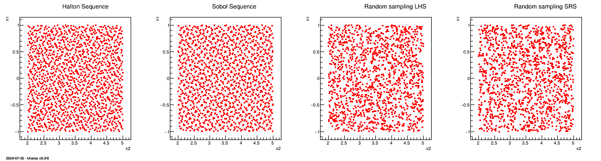
Figure III.10 shows a comparison of the design-of-experiments obtained with both sequences, along with the ones produced with a basic stochastic sampling, following the LHS and SRS "recipes", all when dealing with two uniform attributes. The coverage is clearly more regular in the case of quasi Monte-Carlo sequences which is the origin of their name: low-discrepancy sequences. There are plenty definitions for the notion of discrepancy (see litterature for them) but they all quantify how close the sequence is to a perfect equidistribution of points.

Warning

The Halton sequence has been designed initially to deal with uniform probability law. Extending their use to all probability laws, particularly to infinite-based, it is crucial to set at least lower-bound to these. The Halton sequence first value is indeed 0 and this means that going back from probability space to physical one, would imply value if not properly bounded.

From version 4.3.0, the TQMC will complain about infinite-based law if lower-bounded and from version 4.6.0 it will be fully deprecated.

Figure III.10. Comparison of both quasi Monte-Carlo sequences with both LHS and SRS sampling when dealing with two uniform attributes.

On the other hand, the sparse grid sampling can be very useful for integration purposes and can be used in some of the meta-modelling definition, see, for instance, in Section V.3.1.2. In Uranie we can used the Petras algorithm [Petras2001] to produce these sparse grids, shown for different levels in Figure III.11, that can be compared to regular algorithms ones in Figure III.10 (in both cases, the problem is described with two uniform attributes).

Figure III.11. Comparison of design-of-experiments made with Petras algorithm, using different level values, when dealing with two uniform attributes.

Comparison of design-of-experiments made with Petras algorithm, using different level values, when dealing with two uniform attributes.

In the case of regular sequence, the selected sequence is specified with the second argument option of the class constructor TQMC:

TQMC(tds, option, nCalcul )

First, a pointer to a TDataServer is constructed

tdsqmc = DataServer.TDataServer("tdsQMC", "Test for qMC")
tdsqmc.addAttribute(DataServer.TAttribute("x_{1}", -1.0 , 2.))
tdsqmc.addAttribute(DataServer.TNormalDistribution("x_{2}",  0.0 , 3.))
tdsqmc.addAttribute(DataServer.TAttribute("x_{3}",  1.0, 1.5))

Then, a pointer to a TQMC object is constructed from a TDataServer, of the opted sequence among ("sobol"|"halton"), with the wished size. At the end, the method generateSample() is applied

qmc = Sampler.TQMC(tdsqmc, "sobol", 300)
qmc.generateSample()


III.3. Description of a correlation		III.5. The random fields