

Documentation
/ Manuel utilisateur en Python
: 
| XIV.3. Macros DataServer | ||
|---|---|---|
 | Chapter XIV. Use-cases in python |  |
In a first step, to get accustomed with TDataServer , we propose different macros related to this subject. Since it
constitutes the preliminary and almost mandatory step of a proper use of Uranie, these macros are only for
educational purposes.
The goal of this macro is only to master the objects TAttribute and TDataServer of Uranie. Three
attributes will be created and linked to a TDataServer object, then the log of this object will be
printed to check internal data of this TDataServer.
"""
Example of attribute management
"""
from rootlogon import DataServer

# Define the attribute "x"
px = DataServer.TAttribute("x", -2.0, 4.0)
px.setTitle("#Delta P^{#sigma}")
px.setUnity("#frac{mm^{2}}{s}")

# Define the attribute "y"
py = DataServer.TAttribute("y", 0.0, 1.0)

# Define the DataServer of the study
tds = DataServer.TDataServer("tds", "my first TDS")

# Add the attributes in the DataServer.TDataServer
tds.addAttribute(px)
tds.addAttribute(py)
tds.addAttribute(DataServer.TAttribute("z", 0.25, 0.50))
tds.printLog()
The first attribute "x" is defined on [-2.0, 4.0]; its title is  and unity

px=DataServer.TAttribute("x", -2.0, 4.0);
px.setTitle("#Delta P^{#sigma}");
px.setUnity("#frac{mm^{2}}{s}");
The second attribute "y" is defined on [0.0,1.0]; it will be set with its name as title but without unity.
py=DataServer.TAttribute("y", 0.0, 1.0);
Secondly, a TDataServer object is created and the two attributes x and y
created before are linked to this one.
tds=DataServer.TDataServer("tds", "my first TDS");
tds.addAttribute(px);
tds.addAttribute(py);
Finally, the last attribute z (defined on [0.25,0.50]) is directly added to the TDataServer (its
title will be its name and it will be set without unity) by creating it. An attribute could, indeed, be added to a
TDataServer meanwhile creating it, but then no other information than those available in the constructor would be set.
tds.addAttribute(DataServer.TAttribute("z", 0.25, 0.50));
Then, the log of the TDataServer object is printed.
tds.printLog();
Generally speaking, all Uranie objects have the printLog method which allows to print
internal data of the object.
Processing dataserverAttributes.py...

--- Uranie v4.11/0 --- Developed with ROOT (6.36.06)
                      Copyright (C) 2013-2026 CEA/DES
                      Contact: support-uranie@cea.fr
                      Date: Tue Feb 10, 2026

TDataServer::printLog[]
Name[tds] Title[my first TDS]
Origin[Unknown]
 _sdatafile[]
 _sarchivefile[_dataserver_.root]
*******************************
** TDataSpecification::printLog  ******
**   Name[uheader__tds] Title[Header of my first TDS]
**   relationName[Header of my first TDS]
**   attributs[4]
**** With _listOfAttributes
 Attribute[0/4]
*******************************
** TAttribute::printLog  ******
**    Name[tds__n__iter__]
**   Title[tds__n__iter__]
**   unity[]
**    type[0]
**   share[1]
**   Origin[kIterator]
**   Attribute[kInput]
**   _snote[]
--------------------------------------------------------------------------------------------
--------------------------------------------------------------------------------------------
** - min[] max[]
** - mean[] std[]
**   lowerBound[-1.42387e+64] upperBound[1.42387e+64]
** NOT _defaultValue[]
** NOT _stepValue[]
 ** No Attribute to substitute level[0]
*******************************
 Attribute[1/4]
*******************************
** TAttribute::printLog  ******
**    Name[x]
**   Title[#Delta P^{#sigma}]
**   unity[#frac{mm^{2}}{s}]
**    type[0]
**   share[2]
**   Origin[kAttribute]
**   Attribute[kInput]
**   _snote[]
--------------------------------------------------------------------------------------------
--------------------------------------------------------------------------------------------
** - min[] max[]
** - mean[] std[]
**   lowerBound[-2] upperBound[4]
** NOT _defaultValue[]
** NOT _stepValue[]
 ** No Attribute to substitute level[0]
*******************************
 Attribute[2/4]
*******************************
** TAttribute::printLog  ******
**    Name[y]
**   Title[y]
**   unity[]
**    type[0]
**   share[2]
**   Origin[kAttribute]
**   Attribute[kInput]
**   _snote[]
--------------------------------------------------------------------------------------------
--------------------------------------------------------------------------------------------
** - min[] max[]
** - mean[] std[]
**   lowerBound[0] upperBound[1]
** NOT _defaultValue[]
** NOT _stepValue[]
 ** No Attribute to substitute level[0]
*******************************
 Attribute[3/4]
*******************************
** TAttribute::printLog  ******
**    Name[z]
**   Title[z]
**   unity[]
**    type[0]
**   share[2]
**   Origin[kAttribute]
**   Attribute[kInput]
**   _snote[]
--------------------------------------------------------------------------------------------
--------------------------------------------------------------------------------------------
** - min[] max[]
** - mean[] std[]
**   lowerBound[0.25] upperBound[0.5]
** NOT _defaultValue[]
** NOT _stepValue[]
 ** No Attribute to substitute level[0]
*******************************
** TDataSpecification::fin de printLog *******************************
fin de TDataServer::printLog[]
The objective of this macro is to merge data contained in a TDataServer with data contained in another TDataServer. Both TDataServer
have to contain the same number of patterns. We choose here to merge two TDataServer, loaded from two ASCII files, each
of which contains 9 patterns.
The first ASCII file "tds1.dat" defines the four variables x, dy, z,
theta:
#COLUMN_NAMES: x| dy| z| theta
#COLUMN_TITLES: x_{n}| "#delta y"| ""| #theta
#COLUMN_UNITS: N| Sec| KM/Sec| M^{2}

1 1 11 11
1 2 12 21
1 3 13 31
2 1 21 12
2 2 22 22
2 3 23 32
3 1 31 13
3 2 32 23
3 3 33 33
and the second ASCII file "tds2.dat" defines the four other variables x2,
y, u, ua:
#COLUMN_NAMES: x2| y| u| ua

1 1 102 11
1 2 104 12
1 3 106 13
2 1 202 21
2 2 204 22
2 3 206 23
3 1 302 31
3 2 304 32
3 3 306 33
The merging operation will be executed in the first TDataServer tds1; so it will contain all the
attributes at the end.
"""
Example of data merging
"""
from rootlogon import DataServer

tds1 = DataServer.TDataServer()
tds2 = DataServer.TDataServer()

tds1.fileDataRead("tds1.dat")
print("Dumping tds1")
tds1.Scan("*")

tds2.fileDataRead("tds2.dat")
print("Dumping tds2")
tds2.Scan("*")

tds1.merge(tds2)
print("Dumping merged tds1 and tds2")
tds1.Scan("*", "", "colsize=3 col=9::::::::")
Both TDataServers are filled with ASCII data files with the method filedataRead().
tds1.fileDataRead("tds1.dat");
tds2.fileDataRead("tds2.dat");
Data of the second dataserver tds2 are then merged into the first one.
tds1.merge(tds2);Data are then dumped in the terminal:
tds1.Scan("*");Processing dataserverMerge.py...
--- Uranie v4.11/0 --- Developed with ROOT (6.36.06)
Copyright (C) 2013-2026 CEA/DES
Contact: support-uranie@cea.fr
Date: Tue Feb 10, 2026
Dumping tds1
************************************************************************
* Row * tds1__n__ * x.x * dy.dy * z.z * theta.the *
************************************************************************
* 0 * 1 * 1 * 1 * 11 * 11 *
* 1 * 2 * 1 * 2 * 12 * 21 *
* 2 * 3 * 1 * 3 * 13 * 31 *
* 3 * 4 * 2 * 1 * 21 * 12 *
* 4 * 5 * 2 * 2 * 22 * 22 *
* 5 * 6 * 2 * 3 * 23 * 32 *
* 6 * 7 * 3 * 1 * 31 * 13 *
* 7 * 8 * 3 * 2 * 32 * 23 *
* 8 * 9 * 3 * 3 * 33 * 33 *
************************************************************************
Dumping tds2
************************************************************************
* Row * tds2__n__ * x2.x2 * y.y * u.u * ua.ua *
************************************************************************
* 0 * 1 * 1 * 1 * 102 * 11 *
* 1 * 2 * 1 * 2 * 104 * 12 *
* 2 * 3 * 1 * 3 * 106 * 13 *
* 3 * 4 * 2 * 1 * 202 * 21 *
* 4 * 5 * 2 * 2 * 204 * 22 *
* 5 * 6 * 2 * 3 * 206 * 23 *
* 6 * 7 * 3 * 1 * 302 * 31 *
* 7 * 8 * 3 * 2 * 304 * 32 *
* 8 * 9 * 3 * 3 * 306 * 33 *
************************************************************************
Dumping merged tds1 and tds2
************************************************************************
* Row * tds1__n__ * x.x * dy. * z.z * the * x2. * y.y * u.u * ua. *
************************************************************************
* 0 * 1 * 1 * 1 * 11 * 11 * 1 * 1 * 102 * 11 *
* 1 * 2 * 1 * 2 * 12 * 21 * 1 * 2 * 104 * 12 *
* 2 * 3 * 1 * 3 * 13 * 31 * 1 * 3 * 106 * 13 *
* 3 * 4 * 2 * 1 * 21 * 12 * 2 * 1 * 202 * 21 *
* 4 * 5 * 2 * 2 * 22 * 22 * 2 * 2 * 204 * 22 *
* 5 * 6 * 2 * 3 * 23 * 32 * 2 * 3 * 206 * 23 *
* 6 * 7 * 3 * 1 * 31 * 13 * 3 * 1 * 302 * 31 *
* 7 * 8 * 3 * 2 * 32 * 23 * 3 * 2 * 304 * 32 *
* 8 * 9 * 3 * 3 * 33 * 33 * 3 * 3 * 306 * 33 *
************************************************************************
The objective of this macro is to load two TDataServer objects using two different ways: either with an ASCII file
"pasture.dat" or with a design-of-experiments. Then, we evaluate the analytic function
ModelPasture on this two TDataServer. The data file "pasture.dat" is
written in the "Salome-table" format of Uranie:
#COLUMN_NAMES: time| yield

9 8.93
14 10.8
21 18.59
28 22.33
42 39.35
57 56.11
63 61.73
70 64.62
79 67.08
"""
Example of  data loading with pasture file
"""
from rootlogon import ROOT, DataServer, Sampler, Launcher

C = ROOT.TCanvas("mycanvas", "mycanvas", 1)
ROOT.gROOT.LoadMacro("UserFunctions.C")

tds = DataServer.TDataServer()
tds.fileDataRead("pasture.dat")

tds.getTuple().SetMarkerStyle(8)
tds.getTuple().SetMarkerSize(1.5)
tds.draw("yield:time")

tlf = Launcher.TLauncherFunction(tds, "ModelPasture", "time", "yhat")
tlf.run()

tds.getTuple().SetMarkerColor(ROOT.kBlue)
tds.getTuple().SetLineColor(ROOT.kBlue)

tds.draw("yhat:time", "", "lpsame")

tds2 = DataServer.TDataServer()
tds2.addAttribute(DataServer.TUniformDistribution("time2", 9, 80))

tsamp = Sampler.TSampling(tds2, "lhs", 1000)
tsamp.generateSample()

tds2.getTuple().SetMarkerColor(ROOT.kGreen)
tds2.getTuple().SetLineColor(ROOT.kGreen)
tlf = Launcher.TLauncherFunction(tds2, "ModelPasture", "", "yhat2")
tlf.run()

tds2.draw("yhat2:time2", "", "psame")
tds.draw("yhat:time", "", "lpsame")

ROOT.gPad.SaveAs("pasture.png")
The design ModelPasture is defined in a function
void ModelPasture(Double_t *x, Double_t *y)
{
  Double_t theta1=69.95, theta2=61.68, theta3=-9.209, theta4=2.378;

  y[0] = theta1;
  y[0] -= theta2* TMath::Exp( -1.0 * TMath::Exp( theta3 + theta4 * TMath::Log(x[0])));
}
Which is C++ and is loaded thanks to the function ROOT.gROOT.LoadMacro("UserFunctions.C").
The first TDataServer is filled with the ASCII file "pasture.dat" through the
fileDataRead method
tds.fileDataRead("pasture.dat");
The design is evaluated with the function ModelPasture applied on the input attribute
time, leading to the output attribute named yhat.
tlf=Launcher.TLauncherFunction(tds, "ModelPasture", "time", "yhat");
tlf.run();
A TAttribute, obeying an uniform law on [9;80] is added to the second TDataServer which is filled
with a design-of-experiments of 1000 patterns, using the LHS method.
tsamp=Sampler.TSampling(tds2, "lhs", 1000);
tsamp.generateSample();
The design is now evaluated with this TDataServer on the attribute time2
tlf = Launcher.TLauncherFunction(tds2, "ModelPasture","","yhat2");tlf.setDrawProgressBar(False);
tlf.run();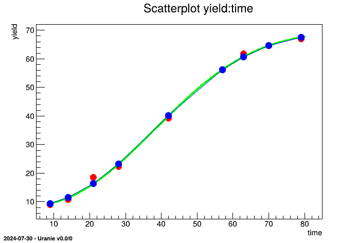
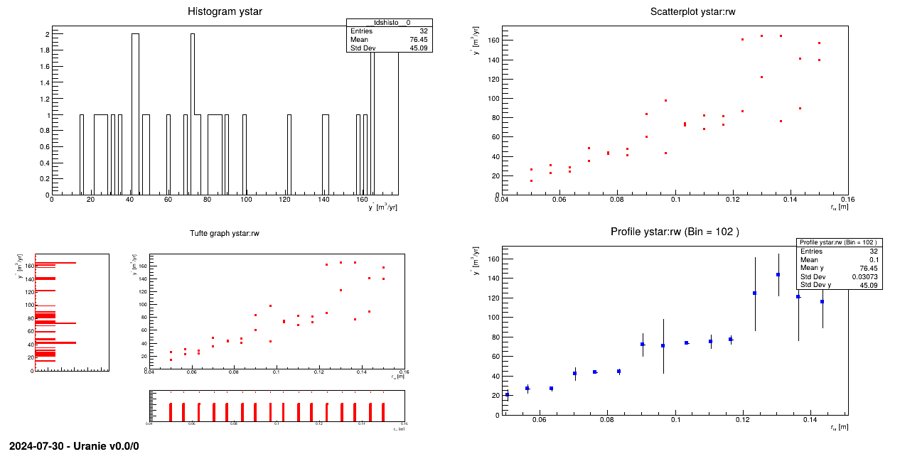
Loading data in a TDataServer, using the "Salome-table" format of Uranie and applying basic visualisation methods on
attributes.
The data file is named "flowrateUniformDesign.dat" and data correspond to an
Uniform design-of-experiments of 32 patterns for a "code" with 8 inputs ( ,
,  ,
,  ,
,  ,
,  ,
,  ,
,  ,
,  ) along with a response
("yhat"). The data file
) along with a response
("yhat"). The data file "flowrateUniformDesign.dat" is in the
"Salome-table" format of Uranie.
#NAME: flowrateborehole
#TITLE: Uniform design of flow rate borehole problem proposed by Ho and Xu(2000)
#COLUMN_NAMES: rw| r| tu| tl| hu| hl| l| kw | ystar
#COLUMN_TITLES: r_{#omega}| r | T_{u} | T_{l} | H_{u} | H_{l} | L | K_{#omega} | y^{*}
#COLUMN_UNITS: m | m | m^{2}/yr | m^{2}/yr | m | m | m | m/yr | m^{3}/yr

0.0500 33366.67  63070.0 116.00 1110.00 768.57 1200.0 11732.14  26.18
0.0500   100.00  80580.0  80.73 1092.86 802.86 1600.0 10167.86  14.46
0.0567   100.00  98090.0  80.73 1058.57 717.14 1680.0 11106.43  22.75
0.0567 33366.67  98090.0  98.37 1110.00 734.29 1280.0 10480.71  30.98
0.0633   100.00 115600.0  80.73 1075.71 751.43 1600.0 11106.43  28.33
0.0633 16733.33  80580.0  80.73 1058.57 785.71 1680.0 12045.00  24.60
0.0700 33366.67  63070.0  98.37 1092.86 768.57 1200.0 11732.14  48.65
0.0700 16733.33 115600.0 116.00  990.00 700.00 1360.0 10793.57  35.36
0.0767   100.0  115600.0  80.73 1075.71 751.43 1520.0 10793.57  42.44
0.0767 16733.33  80580.0  80.73 1075.71 802.86 1120.0  9855.00  44.16
0.0833 50000.00  98090.0  63.10 1041.43 717.14 1600.0 10793.57  47.49
0.0833 50000.00 115600.0  63.10 1007.14 768.57 1440.0 11419.29  41.04
0.0900 16733.33  63070.0 116.00 1075.71 751.43 1120.0 11419.29  83.77
0.0900 33366.67 115600.0 116.00 1007.14 717.14 1360.0 11106.43  60.05
0.0967 50000.00  80580.0  63.10 1024.29 820.00 1360.0  9855.00  43.15
0.0967 16733.33  80580.0  98.37 1058.57 700.00 1120.0 10480.71  97.98
0.1033 50000.00  80580.0  63.10 1024.29 700.00 1520.0 10480.71  74.44
0.1033 16733.33  80580.0  98.37 1058.57 820.00 1120.0 10167.86  72.23
0.1100 50000.00  98090.0  63.10 1024.29 717.14 1520.0 10793.57  82.18
0.1100   100.00  63070.0  98.37 1041.43 802.86 1600.0 12045.00  68.06
0.1167 33366.67  63070.0 116.00  990.00 785.71 1280.0 12045.00  81.63
0.1167   100.00  98090.0  98.37 1092.86 802.86 1680.0  9855.00  72.5
0.1233 16733.33 115600.0  80.73 1092.86 734.29 1200.0 11419.29 161.35
0.1233 16733.33  63070.0  63.10 1041.43 785.71 1680.0 12045.00  86.73
0.1300 33366.67  80580.0 116.00 1110.00 768.57 1280.0 11732.14 164.78
0.1300   100.00  98090.0  98.37 1110.00 820.00 1280.0 10167.86 121.76
0.1367 50000.00  98090.0  63.10 1007.14 820.00 1440.0 10167.86  76.51
0.1367 33366.67  98090.0 116.00 1024.29 700.00 1200.0 10480.71 164.75
0.1433 50000.00  63070.0 116.00  990.00 785.71 1440.0  9855.00  89.54
0.1433 50000.00 115600.0  63.10 1007.14 734.29 1440.0 11732.14 141.09
0.1500 33366.67  63070.0  98.37  990.00 751.43 1360.0 11419.29 139.94
0.1500   100.00 115600.0  80.73 1041.43 734.29 1520.0 11106.43 157.59
"""
Example of data loading file
"""
from rootlogon import ROOT, DataServer

# Create a DataServer.TDataServer
tds = DataServer.TDataServer()
# Load the data base in the DataServer
tds.fileDataRead("flowrateUniformDesign.dat")

# Graph
Canvas = ROOT.TCanvas("c1", "Graph for the Macro loadASCIIFile",
                      5, 64, 1270, 667)
pad = ROOT.TPad("pad", "pad", 0, 0.03, 1, 1)
pad.Draw()
pad.Divide(2, 2)

pad.cd(1)
tds.draw("ystar")
pad.cd(2)
tds.draw("ystar:rw")
pad.cd(3)
tds.drawTufte("ystar:rw")
pad.cd(4)
tds.drawProfile("ystar:rw")

tds.startViewer()
The objective of this macro is to load the ASCII data file "youngsmodulus.dat" and to apply
visualisations on the attribute E with different options. The data file
"youngsmodulus.dat" is in the "Salome-table" format of Uranie.
#NAME: youngsmodulus
#TITLE: Young's Modulus E for the Golden Gate Bridge
#COLUMN_NAMES: E
#COLUMN_TITLES: Young's Modulues
#COLUMN_UNITS: ksi

28900
29200
27400
28700
28400
29900
30200
29500
29600
28400
28300
29300
29300
28100
30200
30200
30300
31200
28800
27600
29600
25900
32000
33400
30600
32700
31300
30500
31300
29000
29400
28300
30500
31100
29300
27400
29300
29300
31300
27500
29400
Data are then exported in header file "youngsmodulus.h" which can be imported in some C file:
// File "youngsmodulus.h" generated by ROOT v5.34/32
// DateTime Tue Nov  3 10:40:13 2015
// DataServer : Name="youngsmodulus" Title="Young's Modulus E for the Golden Gate Bridge" Global Select=""

#define youngsmodulus_nPattern 41

//  Attribute Name="E"
Double_t E[youngsmodulus_nPattern] = {
 2.890000000e+04,
 2.920000000e+04,
 2.740000000e+04,
 2.870000000e+04,
 2.840000000e+04,
 2.990000000e+04,
 3.020000000e+04,
 2.950000000e+04,
 2.960000000e+04,
 2.840000000e+04,
 2.830000000e+04,
 2.930000000e+04,
 2.930000000e+04,
 2.810000000e+04,
 3.020000000e+04,
 3.020000000e+04,
 3.030000000e+04,
 3.120000000e+04,
 2.880000000e+04,
 2.760000000e+04,
 2.960000000e+04,
 2.590000000e+04,
 3.200000000e+04,
 3.340000000e+04,
 3.060000000e+04,
 3.270000000e+04,
 3.130000000e+04,
 3.050000000e+04,
 3.130000000e+04,
 2.900000000e+04,
 2.940000000e+04,
 2.830000000e+04,
 3.050000000e+04,
 3.110000000e+04,
 2.930000000e+04,
 2.740000000e+04,
 2.930000000e+04,
 2.930000000e+04,
 3.130000000e+04,
 2.750000000e+04,
 2.940000000e+04,
};
// End of attribute E

// End of File youngsmodulus.h
"""
Example of young modulus data loading
"""
from rootlogon import ROOT, DataServer

tds = DataServer.TDataServer()
tds.fileDataRead("youngsmodulus.dat")
# gEnv.SetValue("Hist.Binning.1D.x", 10)
# tds.getTuple().Draw("E>>Attribute E(6, 25000, 34000)", "", "text")
# tds.getTuple().Draw("E>>Attribute E(16, 25000, 34000)")

tds.computeStatistic("E")
tds.getAttribute("E").printLog()

tds.exportDataHeader("youngsmodulus.h")

Canvas = ROOT.TCanvas("c1", "Graph for the Macro loadASCIIFile",
                      5, 64, 1270, 667)
pad = ROOT.TPad("pad", "pad", 0, 0.03, 1, 1)
pad.Draw()
pad.Divide(2, 2)

pad.cd(1)
tds.draw("E")
pad.cd(2)
tds.draw("E", "", "nclass=sturges")
pad.cd(3)
tds.draw("E", "", "nclass=scott")
pad.cd(4)
tds.draw("E", "", "nclass=fd")
The TDataServer is filled with the ASCII data file "youngsmodulus.dat" with the method
fileDataRead:
tds.fileDataRead("youngsmodulus.dat");Variable E is then visualised with different options:
tds.draw("E" ,"", "nclass=sturges");
tds.draw("E" ,"", "nclass=scott");
tds.draw("E" ,"", "nclass=fd");
Characteristic values are computed (maximum, minimum, mean and standard deviation) with:
tds.computeStatistic("E");Data are exported in a header file with
tds.exportDataHeader("youngsmodulus.h");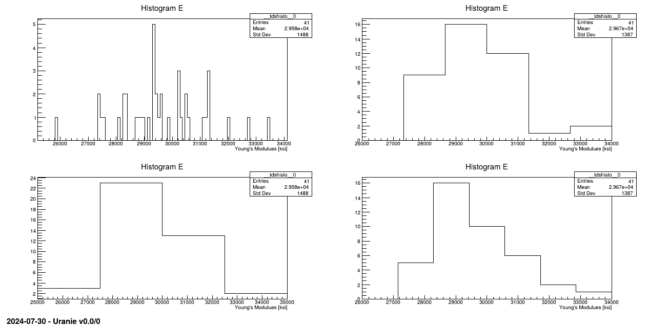
Processing loadASCIIFileYoungsModulus.py...

--- Uranie v4.11/0 --- Developed with ROOT (6.36.06)
                      Copyright (C) 2013-2026 CEA/DES
                      Contact: support-uranie@cea.fr
                      Date: Tue Feb 10, 2026

*******************************
** TAttribute::printLog  ******
**    Name[E]
**   Title[ Young's Modulues]
**   unity[ksi]
**    type[0]
**   share[1]
**   Origin[kAttribute]
**   Attribute[kInput]
**   _snote[]
--------------------------------------------------------------------------------------------
--------------------------------------------------------------------------------------------
** - min[25900] max[33400]
** - mean[29575.6] std[1506.95]
**   lowerBound[-1.42387e+64] upperBound[1.42387e+64]
** NOT _defaultValue[]
** NOT _stepValue[]
 ** No Attribute to substitute level[0]
*******************************
The objective of this macro is to load the ASCII data file ionosphere.dat which defines 34
input variables and one output variable y and applies visualisation on one of
these variables. The data file ionosphere.dat is in the "Salome-table" format of Uranie but
is not shown for convenience.
"""
Example of data loading for Ionosphere dataset
"""
from rootlogon import ROOT, DataServer

tds = DataServer.TDataServer()
tds.fileDataRead("ionosphere.dat")

tds.getAttribute("x28").SetTitle("#Delta P_{e}^{F_{iso}}")

# Graph
Canvas = ROOT.TCanvas("c1", "Graph for the Macro loadASCIIFileIonosphere",
                      5, 64, 1270, 667)
tds.draw("x28")
The TDataServer is filled with ionosphere.dat with the fileDataRead
method
tds.fileDataRead("ionosphere.dat");A new title is set for the variable x28
tds.getAttribute("x28").SetTitle("#Delta P_{e}^{F_{iso}}");This variable is then drawn with its new title
tds.draw("x28");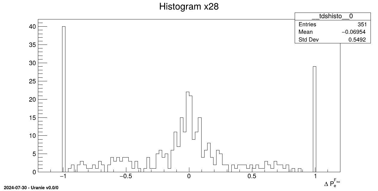
The objective of this macro is to load the ASCII data file cornell.dat which defines seven
input variables and one output variable y on twelve patterns. The input file
cornell.dat is in the "Salome-table" format of Uranie
#NAME: cornell
#TITLE: Dataset Cornell 1990
#COLUMN_NAMES: x1 | x2 | x3 | x4 | x5 | x6 | x7 | y
#COLUMN_TITLES: x_{1} | x_{2} | x_{3} | x_{4} | x_{5} | x_{6} | x_{7} | y

0.00 0.23 0.00 0.00 0.00 0.74 0.03 98.7
0.00 0.10 0.00 0.00 0.12 0.74 0.04 97.8
0.00 0.00 0.00 0.10 0.12 0.74 0.04 96.6
0.00 0.49 0.00 0.00 0.12 0.37 0.02 92.0
0.00 0.00 0.00 0.62 0.12 0.18 0.08 86.6
0.00 0.62 0.00 0.00 0.00 0.37 0.01 91.2
0.17 0.27 0.10 0.38 0.00 0.00 0.08 81.9
0.17 0.19 0.10 0.38 0.02 0.06 0.08 83.1
0.17 0.21 0.10 0.38 0.00 0.06 0.08 82.4
0.17 0.15 0.10 0.38 0.02 0.10 0.08 83.2
0.21 0.36 0.12 0.25 0.00 0.00 0.06 81.4
0.00 0.00 0.00 0.55 0.00 0.37 0.08 88.1
"""
Example of data loading and stat analysis
"""
from rootlogon import DataServer

tds = DataServer.TDataServer()
tds.fileDataRead("cornell.dat")

matCorr = tds.computeCorrelationMatrix("")
matCorr.Print()
The TDataServer is filled with cornell.dat with the fileDataRead method:
tds.fileDataRead("cornell.dat");Then the correlation matrix is computed on all attributes:
matCorr = tds.computeCorrelationMatrix("");Processing loadASCIIFileCornell.py...
--- Uranie v4.11/0 --- Developed with ROOT (6.36.06)
Copyright (C) 2013-2026 CEA/DES
Contact: support-uranie@cea.fr
Date: Tue Feb 10, 2026
8x8 matrix is as follows
| 0 | 1 | 2 | 3 | 4 |
----------------------------------------------------------------------
0 | 1 0.1042 0.9999 0.3707 -0.548
1 | 0.1042 1 0.1008 -0.5369 -0.2926
2 | 0.9999 0.1008 1 0.374 -0.5482
3 | 0.3707 -0.5369 0.374 1 -0.2113
4 | -0.548 -0.2926 -0.5482 -0.2113 1
5 | -0.8046 -0.1912 -0.8052 -0.6457 0.4629
6 | 0.6026 -0.59 0.6071 0.9159 -0.2744
7 | -0.8373 -0.07082 -0.838 -0.7067 0.4938
| 5 | 6 | 7 |
----------------------------------------------------------------------
0 | -0.8046 0.6026 -0.8373
1 | -0.1912 -0.59 -0.07082
2 | -0.8052 0.6071 -0.838
3 | -0.6457 0.9159 -0.7067
4 | 0.4629 -0.2744 0.4938
5 | 1 -0.6564 0.9851
6 | -0.6564 1 -0.7411
7 | 0.9851 -0.7411 1
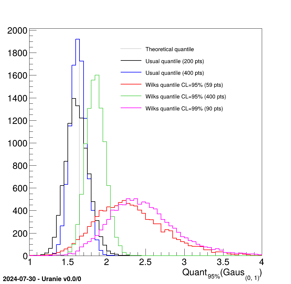
The objective of this macro is to test the classical quantile estimation and compare it to the Wilks estimation for a dummy gaussian distribution. Four different estimations of the 95% quantile value are done (along with one estimation of th 99% quantile) for illustration purposes:
- using the usual method with a 200-points sample.
- using the usual method with a 400-points sample.
- using the Wilks method with a 95% confidence level (with 59-points sample).
- using the Wilks method with a 95% confidence level (with 400-points sample).
- using the Wilks method with a 99% confidence level (with 90-points sample).
"""
Example of quantile estimation (Wilks and not) for illustration purpose
"""
from ctypes import c_double  # For ROOT version greater or equal to 6.20
import numpy as np
from rootlogon import ROOT, DataServer

# Create a DataServer
tds = DataServer.TDataServer("foo", "pouet")
tds.addAttribute("x")  # With one attribute

# Create Histogram to store the quantile values
Q200 = ROOT.TH1F("quantile200", "", 60, 1, 4)
Q200.SetLineColor(1)
Q200.SetLineWidth(2)
Q400 = ROOT.TH1F("quantile400", "", 60, 1, 4)
Q400.SetLineColor(4)
Q400.SetLineWidth(2)
QW95 = ROOT.TH1F("quantileWilks95", "", 60, 1, 4)
QW95.SetLineColor(2)
QW95.SetLineWidth(2)
QW95400 = ROOT.TH1F("quantileWilks95400", "", 60, 1, 4)
QW95400.SetLineColor(8)
QW95400.SetLineWidth(2)
QW99 = ROOT.TH1F("quantileWilks99", "", 60, 1, 4)
QW99.SetLineColor(6)
QW99.SetLineWidth(2)

# Defining the sample size
nb = np.array([200, 400, 59, 90])
proba = 0.95  # Quantile value
CL = np.array([0.95, 0.99])  # CL value for Wilks computation
# Loop over the number of estimation
for iq in range(4):

    # Produce 10000 drawing to get smooth distribution
    for itest in range(10000):

        tds.createTuple()  # Create the tuple to store value
        # Fill it with random drawing of centered gaussian
        for ival in range(nb[iq]):
            tds.getTuple().Fill(ival+1, ROOT.gRandom.Gaus(0, 1))

        # Estimate the quantile...
        quant = c_double(0)  # ROOT.Double for ROOT version lower than 6.20
        if iq < 2:

            # ... with usual methods...
            tds.computeQuantile("x", proba, quant)
            if iq == 0:
                Q200.Fill(quant.value)  # ... on a 200-points sample
            else:
                Q400.Fill(quant.value)  # ... on a 400-points sample
                tds.estimateQuantile("x", proba, quant, CL[iq-1])
                QW95400.Fill(quant.value)  # compute the quantile at 95% CL

        else:

            # ... with the wilks optimised sample
            tds.estimateQuantile("x", proba, quant, CL[iq-2])
            if iq == 2:
                QW95.Fill(quant.value)  # compute the quantile at 95% CL
            else:
                QW99.Fill(quant.value)  # compute the quantile at 99% CL

        # Delete the tuple
        tds.deleteTuple()

# Produce the plot with requested style
ROOT.gStyle.SetOptStat(0)
can = ROOT.TCanvas("Can", "Can", 10, 10, 1000, 1000)
Q400.GetXaxis().SetTitle("Quant_{95%}(Gaus_{(0, 1)})")
Q400.GetXaxis().SetTitleOffset(1.2)
Q400.Draw()
Q200.Draw("same")
QW95.Draw("same")
QW95400.Draw("same")
QW99.Draw("same")

# Add the theoretical estimation
lin = ROOT.TLine()
lin.SetLineStyle(3)
lin.DrawLine(1.645, 0, 1.645, Q400.GetMaximum())

# Add a block of legend
leg = ROOT.TLegend(0.4, 0.6, 0.8, 0.85)
leg.AddEntry(lin, "Theoretical quantile", "l")
leg.AddEntry(Q200, "Usual quantile (200 pts)", "l")
leg.AddEntry(Q400, "Usual quantile (400 pts)", "l")
leg.AddEntry(QW95, "Wilks quantile CL=95% (59 pts)", "l")
leg.AddEntry(QW95400, "Wilks quantile CL=95% (400 pts)", "l")
leg.AddEntry(QW99, "Wilks quantile CL=99% (90 pts)", "l")
leg.SetBorderSize(0)
leg.Draw()
In this macro, a dummy dataserver is created with a single attribute named "x". Four histograms are prepared to store the resulting value. Then the same loop will be used to computed 10000 values of every quantile with different switchs to use one method instead of the other, or to change the number of points in the sample and/or the confidence level. All this is defined in the small part before the loop:
#Defining the sample size
nb=array([200,400,59,90])
quant=ROOT.Double(0.95); #Quantile value
CL =array([0.95, 0.99]);#Confidence level value for the two Wilks computation
Then the computation is performed, first for the usual method (first two iterations of iq), then for
the Wilks estimation (last two iterations of iq). Every computational result is stored in the
corresponding histogram which is finally displayed and shown in the following subsection.
This part shows the complete code used to produce the console display in Section II.4.3.
"""
Example of statistical usage
"""
from rootlogon import DataServer

tdsGeyser = DataServer.TDataServer("geyser", "poet")
tdsGeyser.fileDataRead("geyser.dat")
tdsGeyser.computeStatistic("x1")

print("min(x1)= "+str(tdsGeyser.getAttribute("x1").getMinimum())+";  max(x1)= "
      + str(tdsGeyser.getAttribute("x1").getMaximum())+";  mean(x1)= " +
      str(tdsGeyser.getAttribute("x1").getMean())+";  std(x1)= " +
      str(tdsGeyser.getAttribute("x1").getStd()))
This part shows the complete code used to produce the console display in Section II.4.2.
"""
Example of rank usage for illustration purpose
"""
from rootlogon import DataServer

tdsGeyser = DataServer.TDataServer("geyser", "poet")
tdsGeyser.fileDataRead("geyser.dat")
tdsGeyser.computeRank("x1")
tdsGeyser.computeStatistic("Rk_x1")

print("NPatterns="+str(tdsGeyser.getNPatterns())+";  min(Rk_x1)= " +
      str(tdsGeyser.getAttribute("Rk_x1").getMinimum())+";  max(Rk_x1)= " +
      str(tdsGeyser.getAttribute("Rk_x1").getMaximum()))
This part shows the complete code used to produce the console display in Section II.4.1.
"""
Example of vector normalisation
"""
from rootlogon import DataServer

tdsop = DataServer.TDataServer("foo", "pouet")
tdsop.fileDataRead("tdstest.dat")

# Compute a global normalisation of v, CenterReduced
tdsop.normalize("v", "GCR", DataServer.TDataServer.kCR, True)
# Compute a normalisation of v, CenterReduced (not global but entry by entry)
tdsop.normalize("v", "CR", DataServer.TDataServer.kCR, False)

# Compute a global normalisation of v, Centered
tdsop.normalize("v", "GCent", DataServer.TDataServer.kCentered)
# Compute a normalisation of v, Centered  (not global but entry by entry)
tdsop.normalize("v", "Cent", DataServer.TDataServer.kCentered, False)

# Compute a global normalisation of v, ZeroOne
tdsop.normalize("v", "GZO", DataServer.TDataServer.kZeroOne)
# Compute a normalisation of v, ZeroOne (not global but entry by entry)
tdsop.normalize("v", "ZO", DataServer.TDataServer.kZeroOne, False)

# Compute a global normalisation of v, MinusOneOne
tdsop.normalize("v", "GMOO", DataServer.TDataServer.kMinusOneOne, True)
# Compute a normalisation of v, MinusOneOne (not global but entry by entry)
tdsop.normalize("v", "MOO", DataServer.TDataServer.kMinusOneOne, False)

tdsop.scan("v:vGCR:vCR:vGCent:vCent:vGZO:vZO:vGMOO:vMOO", "",
           "colsize=4 col=2:5::::::::")
This macro should result in this output in console:
*************************************************************************************
*    Row   * Instance *  v *  vGCR *  vCR * vGCe * vCen * vGZO *  vZO * vGMO * vMOO *
*************************************************************************************
*        0 *        0 *  1 * -1.46 *   -1 *   -4 *   -3 *    0 *    0 *   -1 *   -1 *
*        0 *        1 *  2 * -1.09 *   -1 *   -3 *   -3 * 0.12 *    0 * -0.7 *   -1 *
*        0 *        2 *  3 * -0.73 *   -1 *   -2 *   -3 * 0.25 *    0 * -0.5 *   -1 *
*        1 *        0 *  4 * -0.36 *    0 *   -1 *    0 * 0.37 *  0.5 * -0.2 *    0 *
*        1 *        1 *  5 *     0 *    0 *    0 *    0 *  0.5 *  0.5 *    0 *    0 *
*        1 *        2 *  6 * 0.365 *    0 *    1 *    0 * 0.62 *  0.5 * 0.25 *    0 *
*        2 *        0 *  7 * 0.730 *    1 *    2 *    3 * 0.75 *    1 *  0.5 *    1 *
*        2 *        1 *  8 * 1.095 *    1 *    3 *    3 * 0.87 *    1 * 0.75 *    1 *
*        2 *        2 *  9 * 1.460 *    1 *    4 *    3 *    1 *    1 *    1 *    1 *
*************************************************************************************
This part shows the complete code used to produce the console display in Section II.4.3.1.
"""
Example of statistical estimation on vector attributes
"""
from rootlogon import DataServer

tdsop = DataServer.TDataServer("foo", "poet")
tdsop.fileDataRead("tdstest.dat")

# Considering every element of a vector independent from the others
tdsop.computeStatistic("x")
px = tdsop.getAttribute("x")

print("min(x[0])="+str(px.getMinimum(0))+";  max(x[0])="+str(px.getMaximum(0))
      + ";  mean(x[0])="+str(px.getMean(0))+";  std(x[0])="+str(px.getStd(0)))
print("min(x[1])="+str(px.getMinimum(1))+";  max(x[1])="+str(px.getMaximum(1))
      + ";  mean(x[1])="+str(px.getMean(1))+";  std(x[1])="+str(px.getStd(1)))
print("min(x[2])="+str(px.getMinimum(2))+";  max(x[2])="+str(px.getMaximum(2))
      + ";  mean(x[2])="+str(px.getMean(2))+";  std(x[2])="+str(px.getStd(2)))
print("min(xtot)="+str(px.getMinimum(3))+";  max(xtot)="+str(px.getMaximum(3))
      + ";  mean(xtot)="+str(px.getMean(3))+";  std(xtot)="+str(px.getStd(3)))

# Statistic for a single realisation of a vector, not considering other events
tdsop.addAttribute("Min_x", "Min$(x)")
tdsop.addAttribute("Max_x", "Max$(x)")
tdsop.addAttribute("Mean_x", "Sum$(x)/Length$(x)")

tdsop.scan("x:Min_x:Max_x:Mean_x", "", "colsize=5 col=2:::6")
This macro should result in this output in console, split in two parts, the first one being from Uranie's method
min(x[0])= 1;  max(x[0])= 7;  mean(x[0])= 3;  std(x[0])= 3.4641
min(x[1])= 2;  max(x[1])= 8;  mean(x[1])= 4.66667;  std(x[1])= 3.05505
min(x[2])= 3;  max(x[2])= 9;  mean(x[2])= 6.66667;  std(x[2])= 3.21455
min(xtot)= 1;  max(xtot)= 9;  mean(xtot)= 4.77778;  std(xtot)= 3.23179
The second on the other hand results from ROOT's methods (the second part of the code shown above):
*****************************************************
*    Row   * Instance *  x * Min_x * Max_x * Mean_x *
*****************************************************
*        0 *        0 *  1 *     1 *     3 *      2 *
*        0 *        1 *  2 *     1 *     3 *      2 *
*        0 *        2 *  3 *     1 *     3 *      2 *
*        1 *        0 *  7 *     7 *     9 *      8 *
*        1 *        1 *  8 *     7 *     9 *      8 *
*        1 *        2 *  9 *     7 *     9 *      8 *
*        2 *        0 *  1 *     1 *     8 * 4.3333 *
*        2 *        1 *  4 *     1 *     8 * 4.3333 *
*        2 *        2 *  8 *     1 *     8 * 4.3333 *
*****************************************************
This part shows the complete code used to produce the console display in Section II.4.5.1.
"""
Example of correlation matrix computation for vector
"""
from rootlogon import DataServer

tdsop = DataServer.TDataServer("foo", "poet")
tdsop.fileDataRead("tdstest.dat")

# Consider a and x attributes (every element of the vector)
globalOne = tdsop.computeCorrelationMatrix("x:a")
globalOne.Print()

# Consider a and x attributes (cherry-picking a single element of the vector)
focusedOne = tdsop.computeCorrelationMatrix("x[1]:a")
focusedOne.Print()
This macro should result in this output in console.
4x4 matrix is as follows

     |      0    |      1    |      2    |      3    |
---------------------------------------------------------
   0 |          1      0.9449      0.6286       0.189
   1 |     0.9449           1      0.8486         0.5
   2 |     0.6286      0.8486           1      0.8825
   3 |      0.189         0.5      0.8825           1


2x2 matrix is as follows

     |      0    |      1    |
-------------------------------
   0 |          1         0.5
   1 |        0.5           1
This part shows the complete code used to produce the console display in Section II.4.4.1.
"""
Example of quantile estimation for many values at once
"""
from sys import stdout
from ctypes import c_int, c_double
import numpy as np
from rootlogon import ROOT, DataServer

tdsvec = DataServer.TDataServer("foo", "bar")
tdsvec.fileDataRead("aTDSWithVectors.dat")

probas = np.array([0.2, 0.6, 0.8], 'd')
quants = np.array(len(probas)*[0.0], 'd')
tdsvec.computeQuantile("rank", len(probas), probas, quants)

prank = tdsvec.getAttribute("rank")
nbquant = c_int(0)
prank.getQuantilesSize(nbquant)  # (1)
print("nbquant = " + str(nbquant.value))

aproba = c_double(0.8)
aquant = c_double(0)
prank.getQuantile(aproba, aquant)  # (2)
print("aproba = " + str(aproba.value) + ", aquant = " + str(aquant.value))

theproba = np.array(nbquant.value*[0.0], 'd')
thequant = np.array(nbquant.value*[0.0], 'd')
prank.getQuantiles(theproba, thequant)  # (3)
for i_q in range(nbquant.value):
    print("(theproba, thequant)[" + str(i_q) + "] = (" + str(theproba[i_q]) +
          ", " + str(thequant[i_q]) + ")")

allquant = ROOT.vector('double')()
prank.getQuantileVector(aproba, allquant)  # (4)
stdout.write("aproba = " + str(aproba.value) + ", allquant = ")
for quant_i in allquant:
    stdout.write(str(quant_i) + " ")
print("")
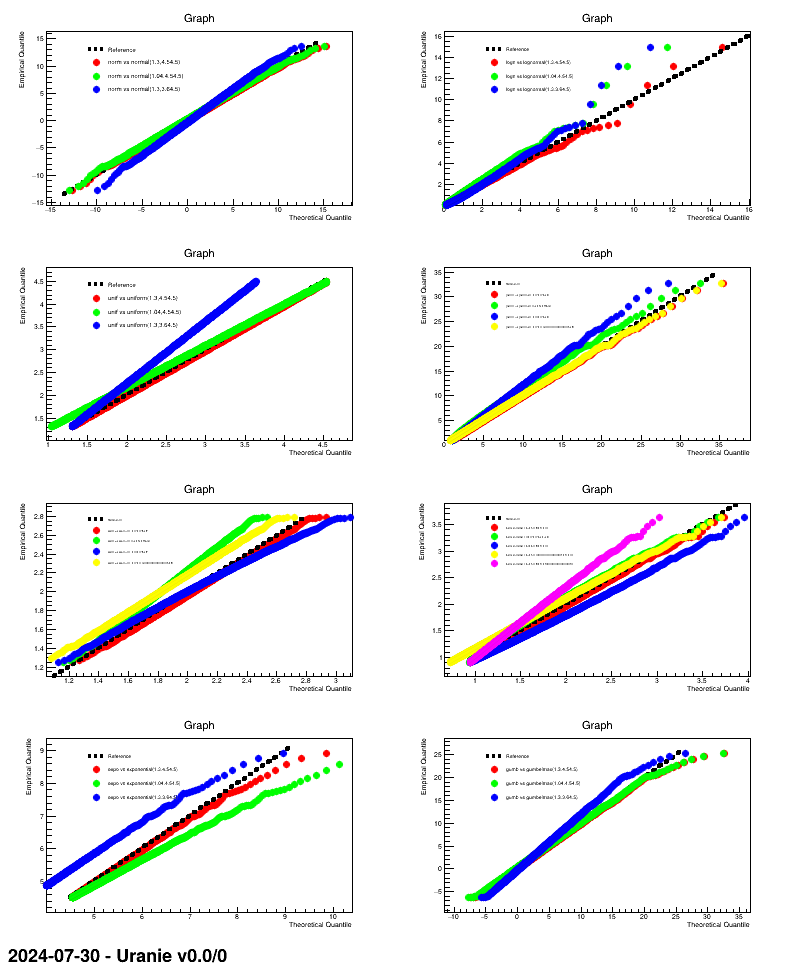
This macro is an example of how to produce QQ-plot for a certain number of randomly-drawn samples, providing the correct parameter values along with modified versions to illustrate the impact.
"""
Example of QQ plot
"""
from rootlogon import ROOT, DataServer, Sampler

# Create a TDS with 8 kind of distributions
p1 = 1.3
p2 = 4.5
p3 = 0.9
p4 = 4.4  # Fixed values for parameters

tds0 = DataServer.TDataServer()
tds0.addAttribute(DataServer.TNormalDistribution("norm", p1, p2))
tds0.addAttribute(DataServer.TLogNormalDistribution("logn", p1, p2))
tds0.addAttribute(DataServer.TUniformDistribution("unif", p1, p2))
tds0.addAttribute(DataServer.TExponentialDistribution("expo", p1, p2))
tds0.addAttribute(DataServer.TGammaDistribution("gamm", p1, p2, p3))
tds0.addAttribute(DataServer.TBetaDistribution("beta", p1, p2, p3, p4))
tds0.addAttribute(DataServer.TWeibullDistribution("weib", p1, p2, p3))
tds0.addAttribute(DataServer.TGumbelMaxDistribution("gumb", p1, p2))

# Create the sample
fsamp = Sampler.TBasicSampling(tds0, "lhs", 200)
fsamp.generateSample()

# Define number of laws, their name and numbers of parameters
nLaws = 8
# number of parameters to put in () for the corresponding law
laws = ["normal", "lognormal", "uniform", "gamma", "weibull",
        "beta", "exponential", "gumbelmax"]
npar = [2, 2, 2, 3, 3, 4, 2, 2]

# Create the canvas
c = ROOT.TCanvas("c1", "", 800, 1000)
# Create the 8 pads
apad = ROOT.TPad("apad", "apad", 0, 0.03, 1, 1)
apad.Draw()
apad.cd()
apad.Divide(2, 4)

# Number of points to compare theoretical and empirical values
nS = 1000
mod = 0.8  # Factor used to artificially change the parameter values

Par = lambda i, n, p, mod: "," + str(p*mod) if n >= i else ""
opt = ""  # option of the drawQQPlot method
for i in range(nLaws):

    # Clean sstr
    test = ""
    # Add nominal configuration
    test += laws[i] + "(" + str(p1) + "," + str(p2) + Par(3, npar[i], p3, 1) \
        + str(p2) + Par(4, npar[i], p4, 1) + ")"
    # Changing par1
    test += ":" + laws[i] + "(" + str(p1*mod) + "," + str(p2) \
        + Par(3, npar[i], p3, 1) + str(p2) + Par(4, npar[i], p4, 1) + ")"
    # Changing par2
    test += ":" + laws[i] + "(" + str(p1) + "," + str(p2*mod) \
        + Par(3, npar[i], p3, 1) + str(p2) + Par(4, npar[i], p4, 1) + ")"
    # Changing par3
    if npar[i] >= 3:
        test += ":" + laws[i] + "(" + str(p1) + "," + str(p2) \
            + Par(3, npar[i], p3, mod) + str(p2) + Par(4, npar[i], p4, 1) + ")"
    # Changing par4
    if npar[i] >= 4:
        test += ":" + laws[i] + "(" + str(p1) + "," + str(p2) \
            + Par(3, npar[i], p3, 1) + str(p2) + Par(4, npar[i], p4, mod) + ")"

    apad.cd(i+1)
    # Produce the plot
    tds0.drawQQPlot(laws[i][:4], test, nS, opt)
The very first step of this macro is to create a sample that will contain a design-of-experiments filled with 200 locations, using
various statistical laws. All the tested laws, are those available in the drawQQPlot
method and they might depend on 2 to 4 parameters, defined a but randomly at the beginning of this piece of code.
## Create a TDS with 8 kind of distributions
p1=1.3; p2=4.5; p3=0.9; p4=4.4; ## Fixed values for parameters

tds0 = DataServer.TDataServer();
tds0.addAttribute(DataServer.TNormalDistribution("norm", p1, p2));
tds0.addAttribute(DataServer.TLogNormalDistribution("logn", p1, p2));
tds0.addAttribute(DataServer.TUniformDistribution("unif", p1, p2));
tds0.addAttribute(DataServer.TExponentialDistribution("expo", p1, p2));
tds0.addAttribute(DataServer.TGammaDistribution("gamm", p1, p2, p3));
tds0.addAttribute(DataServer.TBetaDistribution("beta", p1, p2, p3, p4));
tds0.addAttribute(DataServer.TWeibullDistribution("weib", p1, p2, p3));
tds0.addAttribute(DataServer.TGumbelMaxDistribution("gumb", p1, p2));
Once done, the sample is generated using TBasicSampling object with an LHS algorithm. On top
of this, despite the plot preparation with canvas and pad generation, several variables are set to prepare the
tests, as shown below
## Define number of laws, their name and numbers of parameters
nLaws=8;
laws=["normal", "lognormal", "uniform", "gamma", "weibull", "beta", "exponential", "gumbelmax"];
npar=[2, 2, 2, 3, 3, 4, 2, 2];

## Number of points to compare theoretical and empirical values
nS=1000;
mod=0.8; ## Factor used to artificially change the parameter values
Finally, after the line of hypothesis to be tested is constructed (the first paragraph in the for loop) the
drawQQPlot method is called for every empirical law in the following line.
tds0.drawQQPlot( laws[ilaw][:4], test, nS, opt);
For the first case, when one wants to test the TNormalDistribution "norm" with the known
parameters and a variation of each, it resumes as if this line was run:
tds0.drawQQPlot( "norm", "normal(1.3,4.5):normal(1.04,4.5):normal(1.3,3.6)", nS);The first field is the attribute to be tested, while the second one provides the three hypothesis with which our attribute under investigation will be compared. The third argument is the number of steps to be computed for probabilities. The result of this macro is shown below.
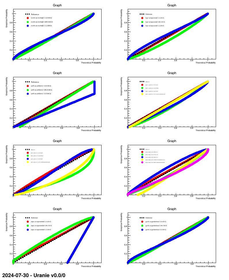
This macro is an example of how to produce PP-plot for a certain number of randomly-drawn samples, providing the correct parameter values along with modified versions to illustrate the impact.
"""
Example of PP plot
"""
from rootlogon import ROOT, DataServer, Sampler

# Create a TDS with 8 kind of distributions
p1 = 1.3
p2 = 4.5
p3 = 0.9
p4 = 4.4  # Fixed values for parameters

tds0 = DataServer.TDataServer()
tds0.addAttribute(DataServer.TNormalDistribution("norm", p1, p2))
tds0.addAttribute(DataServer.TLogNormalDistribution("logn", p1, p2))
tds0.addAttribute(DataServer.TUniformDistribution("unif", p1, p2))
tds0.addAttribute(DataServer.TExponentialDistribution("expo", p1, p2))
tds0.addAttribute(DataServer.TGammaDistribution("gamm", p1, p2, p3))
tds0.addAttribute(DataServer.TBetaDistribution("beta", p1, p2, p3, p4))
tds0.addAttribute(DataServer.TWeibullDistribution("weib", p1, p2, p3))
tds0.addAttribute(DataServer.TGumbelMaxDistribution("gumb", p1, p2))

# Create the sample
fsamp = Sampler.TBasicSampling(tds0, "lhs", 200)
fsamp.generateSample()

# Define number of laws, their name and numbers of parameters
nLaws = 8
# number of parameters to put in () for the corresponding law
laws = ["normal", "lognormal", "uniform", "gamma",
        "weibull", "beta", "exponential", "gumbelmax"]
npar = [2, 2, 2, 3, 3, 4, 2, 2]

# Create the canvas
c = ROOT.TCanvas("c1", "", 800, 1000)
# Create the 8 pads
apad = ROOT.TPad("apad", "apad", 0, 0.03, 1, 1)
apad.Draw()
apad.cd()
apad.Divide(2, 4)

# Number of points to compare theoretical and empirical values
nS = 1000
mod = 0.8  # Factor used to artificially change the parameter values

Par = lambda i, n, p, mod: ","+str(p*mod) if n >= i else ""
opt = ""  # option of the drawPPPlot method
for i in range(nLaws):

    # Clean sstr
    test = ""
    # Add nominal configuration
    test += laws[i] + "(" + str(p1) + "," + str(p2) + Par(3, npar[i], p3, 1) \
        + str(p2) + Par(4, npar[i], p4, 1) + ")"
    # Changing par1
    test += ":" + laws[i] + "(" + str(p1*mod) + "," + str(p2) \
        + Par(3, npar[i], p3, 1) + str(p2) + Par(4, npar[i], p4, 1) + ")"
    # Changing par2
    test += ":" + laws[i] + "(" + str(p1) + "," + str(p2*mod) \
        + Par(3, npar[i], p3, 1) + str(p2) + Par(4, npar[i], p4, 1) + ")"
    # Changing par3
    if npar[i] >= 3:
        test += ":" + laws[i] + "(" + str(p1) + "," + str(p2) \
            + Par(3, npar[i], p3, mod) + str(p2) + Par(4, npar[i], p4, 1) + ")"
    # Changing par4
    if npar[i] >= 4:
        test += ":" + laws[i] + "(" + str(p1) + "," + str(p2) \
            + Par(3, npar[i], p3, 1) + str(p2) + Par(4, npar[i], p4, mod) + ")"

    apad.cd(i+1)
    # Produce the plot
    tds0.drawPPPlot(laws[i][:4], test, nS, opt)
The macro is based on the one discussed in Section XIV.3.15. The only difference is this line
tds0.drawPPPlot( laws[ilaw][:4], test, nS, opt);The call of the drawing method above can be resume, for the first case, like this:
tds0.drawPPPlot( "norm", "normal(1.3,4.5):normal(1.04,4.5):normal(1.3,3.6)", nS);The first field is the attribute to be tested, while the second one provides the three hypothesis with which our attribute under investigation will be compared. The third argument is the number of steps to be computed for probabilities. The result of this macro is shown below.
The goal of this macro is to show how to handle a PCA analysis. It is not much discussed here, as a large description of both methods and concepts is done in Section II.6.
"""
Example of PCA usage (standalone case)
"""
from rootlogon import ROOT, DataServer

# Read the database
tdsPCA = DataServer.TDataServer("tdsPCA", "my TDS")
tdsPCA.fileDataRead("Notes.dat")

# Create the PCA object precising the variables of interest
tpca = DataServer.TPCA(tdsPCA, "Maths:Physics:French:Latin:Music")
tpca.compute()

graphical = True  # do graphs
dumponscreen = True  # or dumping results
showcoordinate = False  # show the points coordinate while dumping results

if graphical:

    # Draw all point in PCA planes
    cPCA = ROOT.TCanvas("cpca", "PCA", 800, 800)
    apad1 = ROOT.TPad("apad1", "apad1", 0, 0.03, 1, 1)
    apad1.Draw()
    apad1.cd()
    apad1.Divide(2, 2)
    apad1.cd(1)
    tpca.drawPCA(1, 2, "Pupil")
    apad1.cd(3)
    tpca.drawPCA(1, 3, "Pupil")
    apad1.cd(4)
    tpca.drawPCA(2, 3, "Pupil")

    # Draw all variable weight in PC definition
    cLoading = ROOT.TCanvas("cLoading", "Loading Plot", 800, 800)
    apad2 = ROOT.TPad("apad2", "apad2", 0, 0.03, 1, 1)
    apad2.Draw()
    apad2.cd()
    apad2.Divide(2, 2)
    apad2.cd(1)
    tpca.drawLoading(1, 2)
    apad2.cd(3)
    tpca.drawLoading(1, 3)
    apad2.cd(4)
    tpca.drawLoading(2, 3)

    # Draw the eigen values in different normalisation
    c = ROOT.TCanvas("cEigenValues", "Eigen Values Plot", 1100, 500)
    apad3 = ROOT.TPad("apad3", "apad3", 0, 0.03, 1, 1)
    apad3.Draw()
    apad3.cd()
    apad3.Divide(3, 1)
    ntd = tpca.getResultNtupleD()
    apad3.cd(1)
    ntd.Draw("eigen:i", "", "lp")
    apad3.cd(2)
    ntd.Draw("eigen_pct:i", "", "lp")
    ROOT.gPad.SetGrid()
    apad3.cd(3)
    ntd.Draw("sum_eigen_pct:i", "", "lp")
    ROOT.gPad.SetGrid()

if dumponscreen:

    nPCused = 5  # 3 to see only the meaningful ones
    PCname = ""
    Cosname = ""
    Contrname = ""
    Variable = "Pupil"
    for iatt in range(1, nPCused+1):
        PCname += "PC_"+str(iatt)+":"
        Cosname += "cosca_"+str(iatt)+":"
        Contrname += "contr_"+str(iatt)+":"

    PCname = PCname[:-1]
    Cosname = Cosname[:-1]
    Contrname = Contrname[:-1]

    print("\n====== EigenValues ======")
    tpca.getResultNtupleD().Scan("*")

    if showcoordinate:
        print("\n====== EigenVectors ======")
        tpca._matEigenVectors.Print()

        print("\n====== New Coordinates ======")
        tdsPCA.scan((Variable+":"+PCname))

    varRes = tpca.getVariableResultNtupleD()
    print("\n====== Looking at variables: Quality of representation ======")
    varRes.Scan(("Variable:"+Cosname))

    print("\n====== Looking at variables: Contribution to axis ======")
    varRes.Scan(("Variable:"+Contrname))

    print("\n====== Looking at events:  Quality of representation ======")
    tdsPCA.scan((Variable+":"+Cosname))

    print("\n====== Looking at events: Contribution to axis ========")
    tdsPCA.scan((Variable+":"+Contrname))
This first part of this macro is described in Section II.6. We will
focus here on the second part, where all the numerical results are dumped on screen. These results are stored in
the dataserver for the points and in a dedicated ntuple for the variable that can be retrieved by calling the method
getVariableResultNtupleD. In both cases, the results can be split into two kinds:
the quality of the representation: it is called "cosca_X" as it is a squared cosinus of the projection of the source under study (point or subject) on the X-th PC.
the contribution to axis: it is called "contr_X" as it is the contribution of the source under study (point or subject) to the definition of the X-th PC.
We start by defining the list of variables that one might want to display
nPCused=5; ## 3 to see only the meaningful ones
PCname=""; Cosname=""; Contrname=""; Variable="Pupil";
for iatt in range(1,nPCused+1) :
##list of PC: PC_1:PC_2:PC_3:PC_4:PC_5
PCname+="PC_"+str(iatt)+":"
##list of quality coeff: cosca_1:cosca_2:cosca_3:cosca_4:cosca_5
Cosname+="cosca_"+str(iatt)+":"
##list of contribution: contr_1:contr_2:contr_3:contr_4:contr_5
Contrname+="contr_"+str(iatt)+":"
pass
PCname=PCname[:-1]; Cosname=Cosname[:-1]; Contrname=Contrname[:-1];
From there, once the variable ntuple is retrieved, one can dump both the quality and contribution coefficients for the variable, here the subjects (it leads to the second and third block in the output shown in Section XIV.3.17.3).
varRes = tpca.getVariableResultNtupleD();
print ("\n=============== Looking at variables: Quality of representation =====================")
varRes.Scan(("Variable:"+Cosname));

print ("\n==================== Looking at variables: Contribution to axis =====================")
varRes.Scan(("Variable:"+Contrname));
Finally, one can do the same for the data points, with the same Scan method (which lead to
the fourth and fifth block in the output shown in Section XIV.3.17.3).
print ("\n================== Looking at events:  Quality of representation ====================")
tdsPCA.scan((Variable+":"+Cosname));

print ("\n===================== Looking at events: Contribution to axis =======================")
tdsPCA.scan((Variable+":"+Contrname));
====== EigenValues ======
************************************************************
*    Row   *       i.i * eigen.eig * eigen_pct * sum_eigen *
************************************************************
*        0 *         1 * 2.8618175 * 57.236350 * 57.236350 *
*        1 *         2 * 1.1506811 * 23.013622 * 80.249973 *
*        2 *         3 * 0.9831407 * 19.662814 * 99.912787 *
*        3 *         4 * 0.0039371 * 0.0787424 * 99.991530 *
*        4 *         5 * 0.0004234 * 0.0084696 *       100 *
************************************************************

====== Looking at variables: Quality of representation ======
************************************************************************************
*    Row   *  Variable *   cosca_1 *   cosca_2 *   cosca_3 *   cosca_4 *   cosca_5 *
************************************************************************************
*        0 *     Maths *  0.649485 *   0.32645 * 0.0235449 * 0.0003614 * 0.0001582 *
*        1 *   Physics *  0.804627 *  0.185581 * 0.0086212 * 0.0010515 * 0.0001193 *
*        2 *    French *  0.574697 *  0.373378 * 0.0509446 * 0.0008976 * 8.252e-05 *
*        3 *     Latin *  0.828562 *  0.157999 * 0.0117556 * 0.0016205 * 6.335e-05 *
*        4 *     Music * 0.0044470 *  0.107272 *  0.888274 * 5.976e-06 * 8.299e-08 *
************************************************************************************

====== Looking at variables: Contribution to axis ======
************************************************************************************
*    Row   *  Variable *   contr_1 *   contr_2 *   contr_3 *   contr_4 *   contr_5 *
************************************************************************************
*        0 *     Maths *  0.226948 *  0.283702 * 0.0239486 * 0.0917987 *  0.373602 *
*        1 *   Physics *  0.281159 *   0.16128 * 0.0087691 *  0.267082 *   0.28171 *
*        2 *    French *  0.200815 *  0.324485 * 0.0518182 *  0.228004 *  0.194878 *
*        3 *     Latin *  0.289523 *  0.137309 * 0.0119572 *  0.411598 *  0.149613 *
*        4 *     Music * 0.0015539 * 0.0932252 *  0.903507 * 0.0015180 * 0.0001959 *
************************************************************************************

====== Looking at events:  Quality of representation ======
************************************************************************************
*    Row   *     Pupil *   cosca_1 *   cosca_2 *   cosca_3 *   cosca_4 *   cosca_5 *
************************************************************************************
*        0 *      Jean * 0.8854534 * 0.0522119 * 0.0619429 * 0.0002655 * 0.0001260 *
*        1 *     Aline * 0.7920409 * 0.0542262 * 0.1530381 * 0.0006354 * 5.916e-05 *
*        2 *     Annie * 0.4784294 * 0.4813342 * 0.0384099 * 0.0018007 * 2.560e-05 *
*        3 *   Monique * 0.8785990 * 0.0024790 * 0.1180158 * 0.0009035 * 2.557e-06 *
*        4 *    Didier * 0.8515216 * 0.1382946 * 0.0079754 * 0.0021718 * 3.640e-05 *
*        5 *     Andre * 0.2465355 * 0.3961581 * 0.3567663 * 9.471e-05 * 0.0004451 *
*        6 *    Pierre * 0.0263090 * 0.7670958 * 0.2060832 * 0.0004625 * 4.925e-05 *
*        7 *  Brigitte * 0.1876629 * 0.5897686 * 0.2211409 * 0.0013390 * 8.836e-05 *
*        8 *   Evelyne * 0.0583185 * 0.3457931 * 0.5953786 * 0.0004600 * 4.957e-05 *
************************************************************************************

====== Looking at events: Contribution to axis ========
************************************************************************************
*    Row   *     Pupil *   contr_1 *   contr_2 *   contr_3 *   contr_4 *   contr_5 *
************************************************************************************
*        0 *      Jean * 0.3012931 * 0.0441856 * 0.0613538 * 0.0656820 * 0.2897335 *
*        1 *     Aline * 0.0618830 * 0.0105370 * 0.0348056 * 0.0360894 * 0.0312404 *
*        2 *     Annie * 0.0401366 * 0.1004284 * 0.0093797 * 0.1098075 * 0.0145176 *
*        3 *   Monique * 0.3784615 * 0.0026558 * 0.1479781 * 0.2828995 * 0.0074454 *
*        4 *    Didier * 0.1484067 * 0.0599446 * 0.0040461 * 0.2751439 * 0.0428726 *
*        5 *     Andre * 0.0348742 * 0.1393737 * 0.1469047 * 0.0097384 * 0.4255425 *
*        6 *    Pierre * 0.0041001 * 0.2973223 * 0.0934888 * 0.0524003 * 0.0518702 *
*        7 *  Brigitte * 0.0157710 * 0.1232678 * 0.0540974 * 0.0817989 * 0.0501849 *
*        8 *   Evelyne * 0.0150734 * 0.2222843 * 0.4479453 * 0.0864396 * 0.0865925 *
************************************************************************************
| |  | |
| XIV.2. Macros Python HowTo |  | XIV.4. Macros Sampler |