Documentation / Manuel utilisateur en Python :

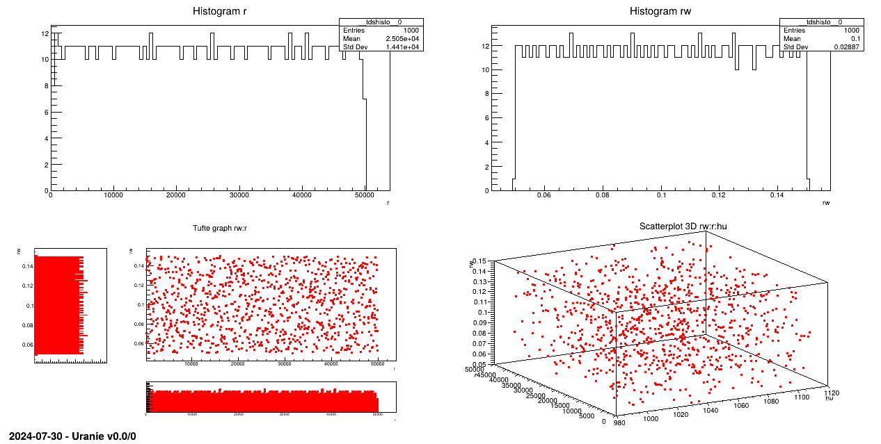
The objective of this macro is to generate a design-of-experiments, of length 100 using the LHS method, with eight random attributes (, , , , , , , ) which obey uniform laws on specific intervals.

"""
Example of simple flowrate DoE generation
"""
from rootlogon import ROOT, DataServer, Sampler

nS = 1000
# Define the DataServer
tds = DataServer.TDataServer("tdsFlowrate", "Design of experiments")

# Add the study attributes
tds.addAttribute(DataServer.TUniformDistribution("rw", 0.05, 0.15))
tds.addAttribute(DataServer.TUniformDistribution("r", 100.0, 50000.0))
tds.addAttribute(DataServer.TUniformDistribution("tu", 63070.0, 115600.0))
tds.addAttribute(DataServer.TUniformDistribution("tl", 63.1, 116.0))
tds.addAttribute(DataServer.TUniformDistribution("hu", 990.0, 1110.0))
tds.addAttribute(DataServer.TUniformDistribution("hl", 700.0, 820.0))
tds.addAttribute(DataServer.TUniformDistribution("l", 1120.0, 1680.0))
tds.addAttribute(DataServer.TUniformDistribution("kw", 9855.0, 12045.0))


# test Generateur de plan d'experience
sampling = Sampler.TSampling(tds, "lhs", nS)
sampling.generateSample()

tds.exportData("_flowrate_sampler_.dat")


# Visualisation
Canvas = ROOT.TCanvas("Canvas", "Graph samplingFlowrate", 5, 64, 1270, 667)
ROOT.gStyle.SetPalette(1)
pad = ROOT.TPad("pad", "pad", 0, 0.03, 1, 1)
pad.Draw()

pad.Divide(2, 2)
pad.cd(1)
tds.draw("r")
pad.cd(2)
tds.draw("rw")
pad.cd(3)
tds.drawTufte("rw:r")
pad.cd(4)
tds.draw("rw:r:hu")

An uniform law is set for each attribute and then, linked to a the TDataServer:

tds.addAttribute(DataServer.TUniformDistribution("rw", 0.05, 0.15));
tds.addAttribute(DataServer.TUniformDistribution("r", 100.0, 50000.0));
tds.addAttribute(DataServer.TUniformDistribution("tu", 63070.0, 115600.0));
tds.addAttribute(DataServer.TUniformDistribution("tl", 63.1, 116.0));
tds.addAttribute(DataServer.TUniformDistribution("hu", 990.0, 1110.0));
tds.addAttribute(DataServer.TUniformDistribution("hl", 700.0, 820.0));
tds.addAttribute(DataServer.TUniformDistribution("l", 1120.0, 1680.0));
tds.addAttribute(DataServer.TUniformDistribution("kw", 9855.0, 12045.0));

The sampling is generated with the LHS method:

sampling=Sampler.TSampling(tds, "lhs", nS);   
sampling.generateSample();

Data are exported in an ASCII file:

tds.exportData("_flowrate_sampler_.dat");

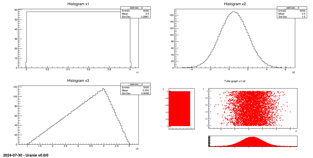
Generate a design-of-experiments of 5000 patterns, using the LHS method, with three random attributes:

 """
Example of LHS DoE sampling
"""
from rootlogon import ROOT, DataServer, Sampler

# Create a DataServer.TDataServer
tds = DataServer.TDataServer()
# Fill the DataServer with the three attributes of the study
tds.addAttribute(DataServer.TUniformDistribution("x1", 3., 4.))
tds.addAttribute(DataServer.TNormalDistribution("x2", 0.5, 1.5))
tds.addAttribute(DataServer.TTriangularDistribution("x3", 1., 5., 4.))


# Generate the sampling from the DataServer.TDataServer
sampling = Sampler.TSampling(tds, "lhs", 5000)
sampling.generateSample()

tds.StartViewer()

# Graph
Canvas = ROOT.TCanvas("c1", "Graph for the Macro sampling", 5, 64, 1270, 667)
pad = ROOT.TPad("pad", "pad", 0, 0.03, 1, 1)
pad.Draw()
pad.Divide(2, 2)

pad.cd(1)
tds.Draw("x1")
pad.cd(2)
tds.Draw("x2")
pad.cd(3)
tds.Draw("x3")
pad.cd(4)
tds.drawTufte("x1:x2")

Laws are set for each attribute and linked to a TDataServer:

tds.addAttribute(DataServer.TUniformDistribution("x1", 3., 4.));
tds.addAttribute(DataServer.TNormalDistribution("x2", 0.5, 1.5));
tds.addAttribute(DataServer.TTriangularDistribution("x3", 1., 5., 4.));

The sampling is generated with the LHS method!

sampling=Sampler.TSampling(tds, "lhs", 5000);   
sampling.generateSample();

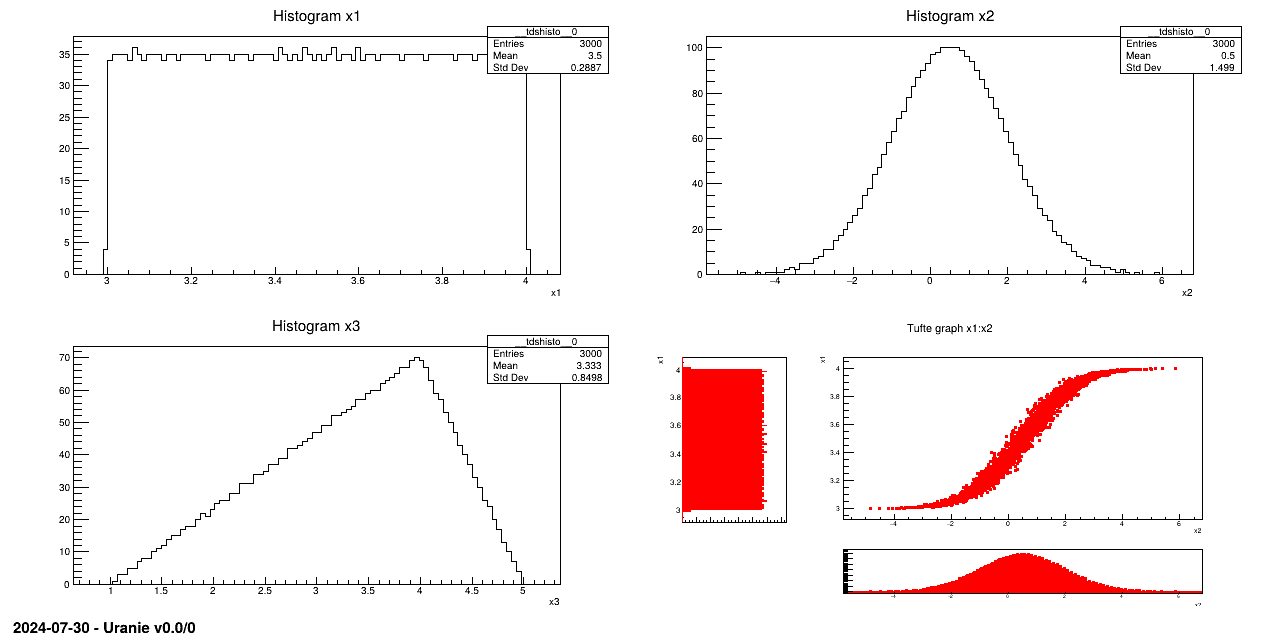
Generate a design-of-experiments, of 3000 patterns using the LHS method, with 3 random attributes and taking into account a correlation between the first two attributes. This correlation, equals to 0.99, is computed using the rank values (the Spearmann definition, c.f. Section III.3 and in [Metho] for more details).

"""
Example of simple LHS correlated DoE generation
"""
from rootlogon import ROOT, DataServer, Sampler

# Create a DataServer.TDataServer
tds = DataServer.TDataServer()
# Fill the DataServer with the three attributes of the study
tds.addAttribute(DataServer.TUniformDistribution("x1", 3., 4.))
tds.addAttribute(DataServer.TNormalDistribution("x2", 0.5, 1.5))
tds.addAttribute(DataServer.TTriangularDistribution("x3", 1., 5., 4.))

# Generate the sampling from the DataServer.TDataServer
sampling = Sampler.TSampling(tds, "lhs", 3000)
sampling.setUserCorrelation(0, 1, 0.99)
sampling.generateSample()

tds.exportData("toto.dat", "x1:x3")
tds.exportDataHeader("toto.h", "x1:x2")

# Graph
Canvas = ROOT.TCanvas("c1", "Graph samplingCorrelation", 5, 64, 1270, 667)
pad = ROOT.TPad("pad", "pad", 0, 0.03, 1, 1)
pad.Draw()
pad.Divide(2, 2)

pad.cd(1)
tds.Draw("x1")
pad.cd(2)
tds.Draw("x2")
pad.cd(3)
tds.Draw("x3")
pad.cd(4)
tds.drawTufte("x1:x2")

Laws are set for each attribute and linked to a TDataServer:

tds.addAttribute(DataServer.TUniformDistribution("x1", 3., 4.));
tds.addAttribute(DataServer.TNormalDistribution("x2", 0.5, 1.5));
tds.addAttribute(DataServer.TTriangularDistribution("x3", 1., 5., 4.));

The sampling is generated with the LHS method and a correlation is set between the two first attributes:

sampling=Sampler.TSampling(tds, "lhs", 3000);
sampling.setUserCorrelation(0, 1, 0.99);      
sampling.generateSample();

Data are partially exported in an ASCII file and a header file:

tds.exportData("toto.dat","x1:x3");
tds.exportDataHeader("toto.h","x1:x2");

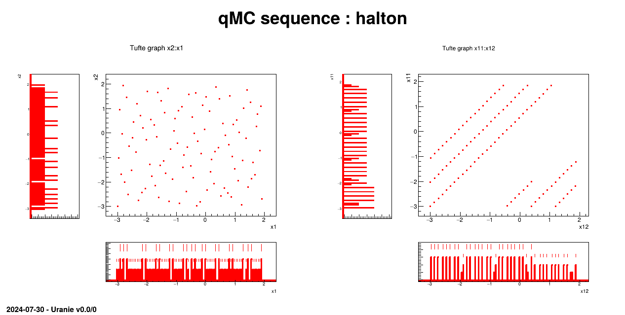
Generate a design-of-experiments of 100 patterns using quasi Monte-Carlo methods ("Halton" or "Sobol") with 12 random attributes, following an uniform law on [3.,2.]. All these information are introduced by variables which will be used by the rest of the macro.

"""
Example of quasi monte-carlo generation
"""
from rootlogon import ROOT, DataServer, Sampler

# Parameters
nSampler = 100
sQMC = "halton"  # halton / sobol
nVar = 12

# Create a DataServer.TDataServer
tds = DataServer.TDataServer()

# Fill the DataServer with the nVar attributes of the study
for i in range(nVar):
    tds.addAttribute(DataServer.TUniformDistribution("x"+str(i+1), -3.0, 2.0))

# Generate the quasi Monte-Carlo sequence from the DataServer.TDataServer
qmc = Sampler.TQMC(tds, sQMC, nSampler)
qmc.generateSample()

# Visualisation
Canvas = ROOT.TCanvas("c1", "Graph for the Macro qmc", 5, 64, 1270, 667)
Canvas.Range(0, 0, 25, 18)

pl = ROOT.TPaveLabel(1, 16.3, 24, 17.5, "qMC sequence : "+sQMC, "br")
pl.SetBorderSize(0)
pl.Draw()

pad1 = ROOT.TPad("pad1", "Determ", 0.02, 0.05, 0.48, 0.88)
pad2 = ROOT.TPad("pad2", "Stoch", 0.52, 0.05, 0.98, 0.88)
pad1.Draw()
pad2.Draw()

pad1.cd()
tds.drawTufte("x2:x1")
pad2.cd()
tds.drawTufte("x11:x12")

Laws are set for each attribute and linked to a TDataServer:

for i in range(nVar) : tds.addAttribute(DataServer.TUniformDistribution( "x"+str(i+1), -3.0, 2.0));

The sampling is generated with the QMC method and a correlation is set between the two first attributes:

qmc=Sampler.TQMC(tds, sQMC, nSampler);
qmc.generateSample();

The rest of the code is used to produce a plot.

The objective is to perform three basic samplings, the first with 10000 variables on 10 patterns using a SRS method, the second with 10000 variables on 10 patterns with a LHS method and the third with 10000 variables on 5000 patterns with a SRS method. Each sampling is related to a specific function, and these three functions are run in a fourth one.

"""
Example of simple DoE generations
"""
from rootlogon import ROOT, DataServer, Sampler


def test_big_sampling():
    """Produce a large sample."""
    tds = DataServer.TDataServer()
    print("    - Creating attributes...")
    for i in range(4000):
        tds.addAttribute(DataServer.TUniformDistribution("x_"+str(i), 0., 1.))
    sam = Sampler.TBasicSampling(tds, "srs", 5000)
    print("    - Starting sampling...")
    sam.generateSample()


def test_small_srs_sampling():
    """Produce a small srs sample."""
    tds = DataServer.TDataServer()
    print("    - Creating attributes...")
    for i in range(10000):
        tds.addAttribute(DataServer.TUniformDistribution("x_"+str(i), 0., 1.))
    sam = Sampler.TBasicSampling(tds, "srs", 10)
    print("    - Starting sampling...")
    sam.generateSample()


def test_small_lhs_sampling():
    """Produce a small lhs sample."""
    tds = DataServer.TDataServer()
    print("    - Creating attributes...")
    for i in range(10000):
        tds.addAttribute(DataServer.TUniformDistribution("x_"+str(i), 0., 1.))
    sam = Sampler.TBasicSampling(tds, "lhs", 10)
    print("    - Starting sampling...")
    sam.generateSample()


print("***************************************************")
print(" ** Test small SRS sampling (10000 attributes, 10 data)")
test_small_srs_sampling()
print("***************************************************")
ROOT.gROOT.ls()

print("***************************************************")
print(" ** Test small LHS sampling (10000 attributes, 10 data)")
test_small_lhs_sampling()
print("***************************************************")
ROOT.gROOT.ls()

print("***************************************************")
print(" ** Test big sampling (4000 attributes, 5000 data)")
test_big_sampling()
print("***************************************************")
ROOT.gROOT.ls()

This part shows the complete code used to produce the console display in Section III.6.3.3.

"""
Example of regular OAT generation
"""
from rootlogon import DataServer, Sampler

# step 1
tds = DataServer.TDataServer("tdsoat", "Data server for simple OAT design")
tds.addAttribute(DataServer.TAttribute("x1"))
tds.addAttribute(DataServer.TAttribute("x2"))

# step 2
tds.getAttribute("x1").setDefaultValue(0.0)
tds.getAttribute("x2").setDefaultValue(10.0)

# step 3
oatSampler = Sampler.TOATDesign(tds, "regular", 4)

# step 4
use_percentage = True
oatSampler.setRange("x1", 2.0)
oatSampler.setRange("x2", 40.0, use_percentage)

# step 5
oatSampler.generateSample()

# display
tds.scan()

This part shows the complete code used to produce the console display in Section III.6.3.4.

"""
Example of OAT generation with random locations
"""
from rootlogon import ROOT, DataServer, Sampler

# step 1
tds = DataServer.TDataServer("tdsoat", "Data server for simple OAT design")
tds.addAttribute(DataServer.TUniformDistribution("x1", -5.0, 5.0))
tds.addAttribute(DataServer.TNormalDistribution("x2", 11.0, 1.0))

# step 2
tds.getAttribute("x1").setDefaultValue(0.0)
tds.getAttribute("x2").setDefaultValue(10.0)

# step 3
oatSampler = Sampler.TOATDesign(tds, "lhs", 1000)

# step 4
use_percentage = True
oatSampler.setRange("x1", 2.0)
oatSampler.setRange("x2", 40.0, use_percentage)

# step 5
oatSampler.generateSample()

c = ROOT.TCanvas("can", "can", 10, 32, 1200, 600)
apad = ROOT.TPad("apad", "apad", 0, 0.03, 1, 1)
apad.Draw()
apad.Divide(2, 1)
apad.cd(1)
tds.draw("x1", "__modified_att__ == 1")
apad.cd(2)
tds.draw("x2", "__modified_att__ == 2")

This part shows the complete code used to produce the console display in Section III.6.3.5.

"""
Example of OAT multi start generation
"""
from rootlogon import DataServer, Sampler

# step 1
tds = DataServer.TDataServer("tdsoat", "Data server for simple OAT design")
tds.fileDataRead("myNominalValues.dat")

# step 3
oatSampler = Sampler.TOATDesign(tds)

# step 4
use_percentage = True
oatSampler.setRange("x1", 2.0)
oatSampler.setRange("x2", 40.0, use_percentage)

# step 5
oatSampler.generateSample()

# display
tds.scan()

This part shows the complete code used to produce the console display in Section III.6.3.6.

"""
Example of OAT generation with range options
"""
from rootlogon import DataServer, Sampler

# step 1
tds = DataServer.TDataServer("tds", "Data server for simple OAT design")
tds.fileDataRead("myNominalValues.dat")

# step 3
oatSampler = Sampler.TOATDesign(tds)

# step 4
use_percentage = True
oatSampler.setRange("x1", "rx1")
oatSampler.setRange("x2", 40.0, use_percentage)

# step 5
oatSampler.generateSample()

# display
tds.scan()

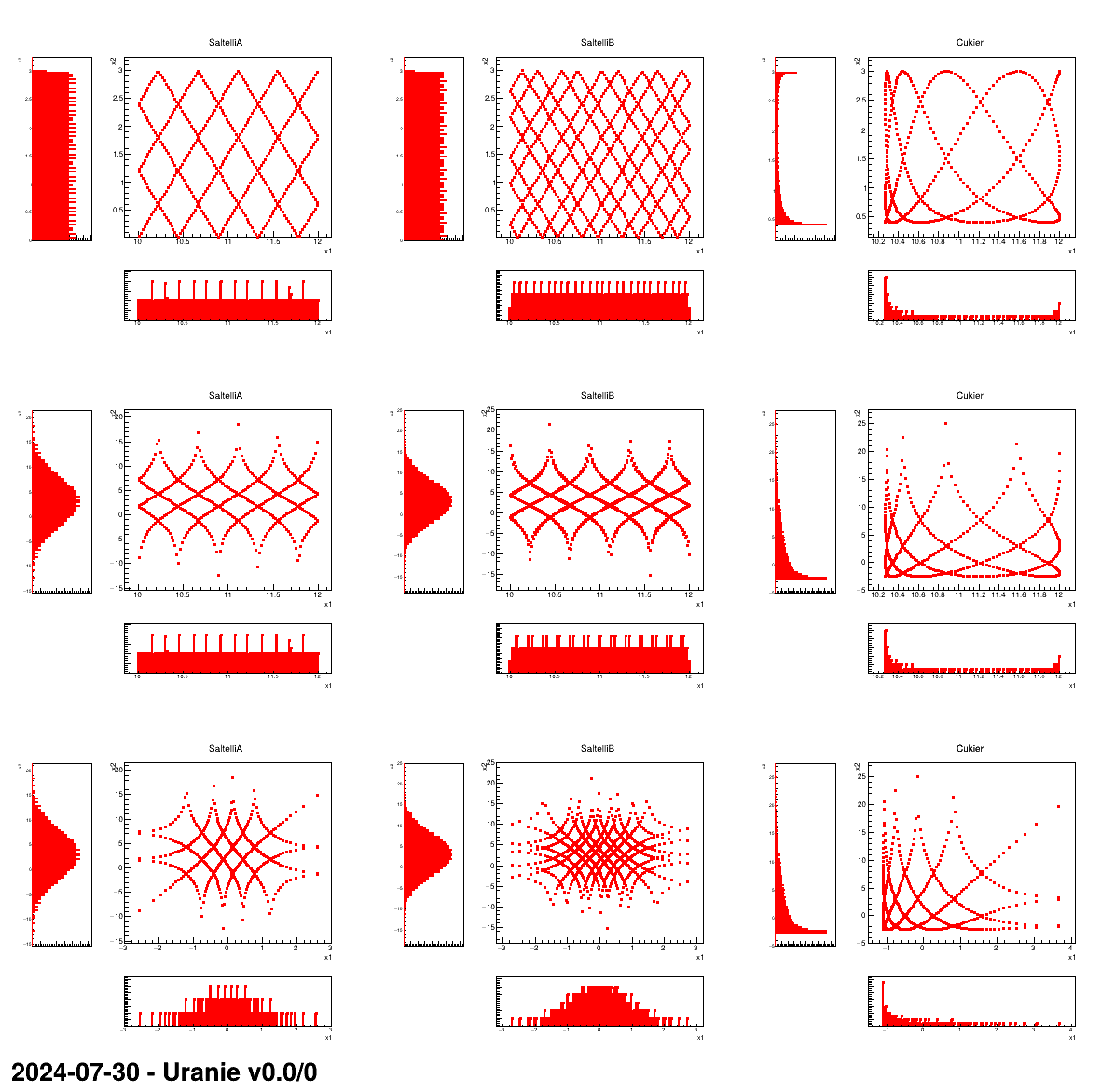
This macro shows the usage of the TSpaceFilling class and the resulting design-of-experiments in three simple dataserver cases:

For each of these configurations (represented in the following plot by a line), the three available algorithms are also tested. They are called:

This kind of design-of-experiments is not intented to be used regurlarly, it is requested only by few mechanisms like the FAST and RBD methods which rely on fourier transformations. This macro and, above all, the following plot, is made mainly for illustration purpose.

"""
Example of space filling DoE
"""
from rootlogon import ROOT, DataServer, Sampler


def generate_and_draw_it(l_pad, l_tds, l_tsp, l_nb, l_title):
    """Delete the tuple, generate a sample and draw the plot."""

    l_pad.cd(l_nb+1)
    l_tds.deleteTuple()
    l_tsp.generateSample()
    l_tds.drawTufte("x2:x1")
    l_pad.GetPad(l_nb+1).GetPrimitive("TPave").SetLabel("")
    ROOT.gPad.GetPrimitive("htemp").SetTitle(l_title)
    ROOT.gPad.Modified()


# Attributes
att1 = DataServer.TUniformDistribution("x1", 10, 12)
att2 = DataServer.TUniformDistribution("x2", 0, 3)
nor1 = DataServer.TNormalDistribution("x1", 0, 1)
nor2 = DataServer.TNormalDistribution("x2", 3, 5)

# Pointer to DataServer and Samplers
tds = [0., 0., 0.]
tsp = [0., 0., 0., 0., 0., 0., 0., 0., 0.]
algoname = ["SaltelliA", "SaltelliB", "Cukier"]

# Canvas to produce the 3x3 plot
Can = ROOT.TCanvas("Can", "Can", 10, 32, 1200, 1200)
pad = ROOT.TPad("pad", "pad", 0, 0.03, 1, 1)
pad.Draw()
pad.Divide(3, 3)
ct = 0

for itds in range(3):

    # Create a DataServer to store new configuration
    # (UnivsUni, GausvsUni, Gaus vs Gaus)
    tds[itds] = DataServer.TDataServer("test", "test")
    if itds == 0:
        tds[itds].addAttribute(att1)
        tds[itds].addAttribute(att2)
    if itds == 1:
        tds[itds].addAttribute(att1)
        tds[itds].addAttribute(nor2)
    if itds == 2:
        tds[itds].addAttribute(nor1)
        tds[itds].addAttribute(nor2)

    # Looping over the 3 spacefilling algo available
    for ialg in range(3):
        # Instantiate the sampler
        if ialg == 0:
            tsp[ct] = Sampler.TSpaceFilling(tds[itds], "srs", 1000,
                                            Sampler.TSpaceFilling.kSaltelliA)
        if ialg == 1:
            tsp[ct] = Sampler.TSpaceFilling(tds[itds], "srs", 1000,
                                            Sampler.TSpaceFilling.kSaltelliB)
        if ialg == 2:
            tsp[ct] = Sampler.TSpaceFilling(tds[itds], "srs", 1000,
                                            Sampler.TSpaceFilling.kCukier)

        # Draw with correct legend
        generate_and_draw_it(pad, tds[itds], tsp[ct], ct, algoname[ialg])
        ct = ct+1

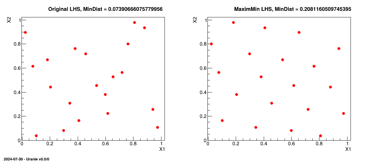
This macro shows the usage of the TMaxiMinLHS class in the case where it is used with an already provided LHS grid. The class itself can generate a LHS grid from scratch (on which the simulated annealing algorithm will be applied to get a maximin grid) but the idea for this macro is to do this procedure in two steps to be able to compare the original LHS grid and the results of the optimisation. The orginal design-of-experiments is done with two uniformly-distributed variables.

The resulting design-of-experiments presented is presented side-by-side with the original one and the mindist criterion calculated is displayed on top of both grid, for illustration purpose.

"""
Example of maximin lhs sample generation
"""
from rootlogon import ROOT, DataServer, Sampler


def niceplot(l_tds, l_lat, l_title):
    """Generate the grid plot."""

    l_tds.getTuple().SetMarkerStyle(20)
    l_tds.getTuple().SetMarkerSize(1)
    l_tds.Draw("X2:X1")
    tit = "MinDist = "+str(Sampler.TMaxiMinLHS.getMinDist(l_tds.getMatrix()))
    ROOT.gPad.GetPrimitive("__tdshisto__0").SetTitle("")
    ROOT.gPad.GetPrimitive("__tdshisto__0").GetXaxis().SetRangeUser(0., 1.)
    ROOT.gPad.GetPrimitive("__tdshisto__0").GetYaxis().SetRangeUser(0., 1.)
    l_lat.DrawLatex(0.25, 0.94, l_title+", "+tit)


# Canvas to produce the 2x1 plot to compare LHS designs
Can = ROOT.TCanvas("Can", "Can", 10, 32, 1200, 550)
pad = ROOT.TPad("pad", "pad", 0, 0.03, 1, 1)
pad.Draw()
pad.Divide(2, 1)

size = 20  # Size of the samples to be produced
lat = ROOT.TLatex()
lat.SetNDC()
lat.SetTextSize(0.038)  # To write titles

# Create dataserver and define the attributes
tds = DataServer.TDataServer("tds", "pouet")
tds.addAttribute(DataServer.TUniformDistribution("X1", 0, 1))
tds.getAttribute("X1").delShare()  # state to tds that it owns it
tds.addAttribute(DataServer.TUniformDistribution("X2", 0, 1))
tds.getAttribute("X2").delShare()  # state to tds that it owns it

# Generate the original LHS grid
sampl = Sampler.TSampling(tds, "lhs", size)
sampl.generateSample()

# Display it
pad.cd(1)
niceplot(tds, lat, "Original LHS")

# Transform the grid in a maximin LHD
# Set initial temperature to 0.1, c factor to 0.99 and loop limitations to 300
# following official recommandation in methodology manual
maxim = Sampler.TMaxiMinLHS(tds, size, 0.1, 0.99, 300, 300)
maxim.generateSample()

# Display it
pad.cd(2)
niceplot(tds, lat, "MaximMin LHS")

The macro very much looks like any other design-of-experiments generating macro above: the dataserver is created and the problem is defined along with the input variables. A LHS grid is generated through the use of TSampling and display in the first part of the canvas, calling a generic function niceplot defined on top of this macro. The new part comes with the following lines:

# Transform the grid in a maximin LHD
# Set initial temperature to 0.1, c factor to 0.99 and loop limitations to 300 following official recommandation in methodology manual
maxim=Sampler.TMaxiMinLHS(tds, size, 0.1, 0.99, 300, 300);  
maxim.generateSample();

The construction line of a TMaxiMinLHS is a bit different from the usual TSampling object: on top of a pointer to the dataserver, it requires the size of the grid to be generated and the main characteristic of the simulated annealing method to be used for the optimisation of the mindist criteria. A more complete discussion is done on this subject in [metho]

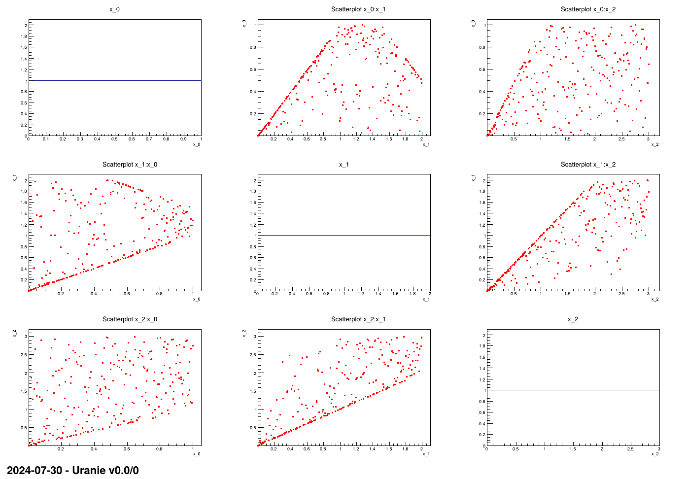
This macro shows the usage of the TConstrLHS class when one wants to create a constrained LHS with three linear constraints. In order to illustate the concept, it is applied on three input variables drawn from uniform distribution with well-thought boundaries (as the concept of the LHS is to have nicely distributed marginals).

"""
Example of constrained lhs with linear constraints
"""
import numpy as np
from rootlogon import ROOT, DataServer, Sampler


def nicegrid(l_tds, l_can):
    """Generate the grid plot."""

    l_ns = l_tds.getNPatterns()
    l_nx = l_tds.getNAttributes()
    l_tds.drawPairs()

    all_h = []
    ROOT.gStyle.SetOptStat(0)
    for iatt in range(l_nx):

        l_can.GetPad(iatt*(l_nx+1)+1).cd()
        att = l_tds.getAttribute(iatt)
        a_name = att.GetName()
        all_h.append(ROOT.TH1F(a_name+"_histo", a_name+";x_"+str(iatt),
                               l_ns, att.getLowerBound(), att.getUpperBound()))
        l_tds.Draw(a_name+">>"+a_name+"_histo", "", "goff")
        all_h[iatt].Draw()

    return all_h


# Canvas to produce the pair plot
Can = ROOT.TCanvas("Can", "Can", 10, 32, 1400, 1000)
apad = ROOT.TPad("apad", "apad", 0, 0.03, 1, 1)
apad.Draw()
apad.cd()

ns = 250  # Size of the samples to be produced
nx = 3

# Create dataserver and define the attributes
tds = DataServer.TDataServer("tds", "pouet")
for i in range(nx):

    tds.addAttribute(DataServer.TUniformDistribution("x_"+str(i), 0, i+1))
    tds.getAttribute("x_"+str(i)).delShare()

ROOT.gROOT.LoadMacro("ConstrFunctions.C")

# Generate the constr lhs
constrlhs = Sampler.TConstrLHS(tds, ns)
inputs = np.array([1, 0, 2, 1], dtype='i')
constrlhs.addConstraint(ROOT.Linear, 2, len(inputs), inputs)
constrlhs.generateSample()

# Do the plot
ListOfDiag = nicegrid(tds, apad)

The very beginning of these macros is the nicegrid method which is here only to show the nice marginal distributions and the scatter plots. One can clearly skip this part to focus on the rest in the main function.

The macro very much looks like any other design-of-experiments generating macro above: the dataserver is created along with the canvas object and the problem is defined along with the input variables and the number of locations to be produced. Once done, then the TConstrLHS instance is created with the four following lines:

# Generate the constr lhs
constrlhs = Sampler.TConstrLHS(tds, ns)
inputs = numpy.array([1, 0, 2, 1], dtype= i )
constrlhs.addConstraint(ROOT.Linear, 2, len(inputs), inputs)
constrlhs.generateSample()

The constructor is pretty obvious, as it takes only the dataserver object and the number of locations. Once created the main method to be called is the addConstraint function which has been largely discussed in Section III.2.4. The first argument of this method is the pointer to the C++ function which has been included in our macro through a line juste before the sampler creation:

ROOT.gROOT.LoadMacro("ConstrFunctions.C")

which contains the Linear function. The rest of the argument are the number of constraints, the size of the list of parameters and its content. Finally the nicegrid method is called to produce the nice plot shown in Figure XIV.15

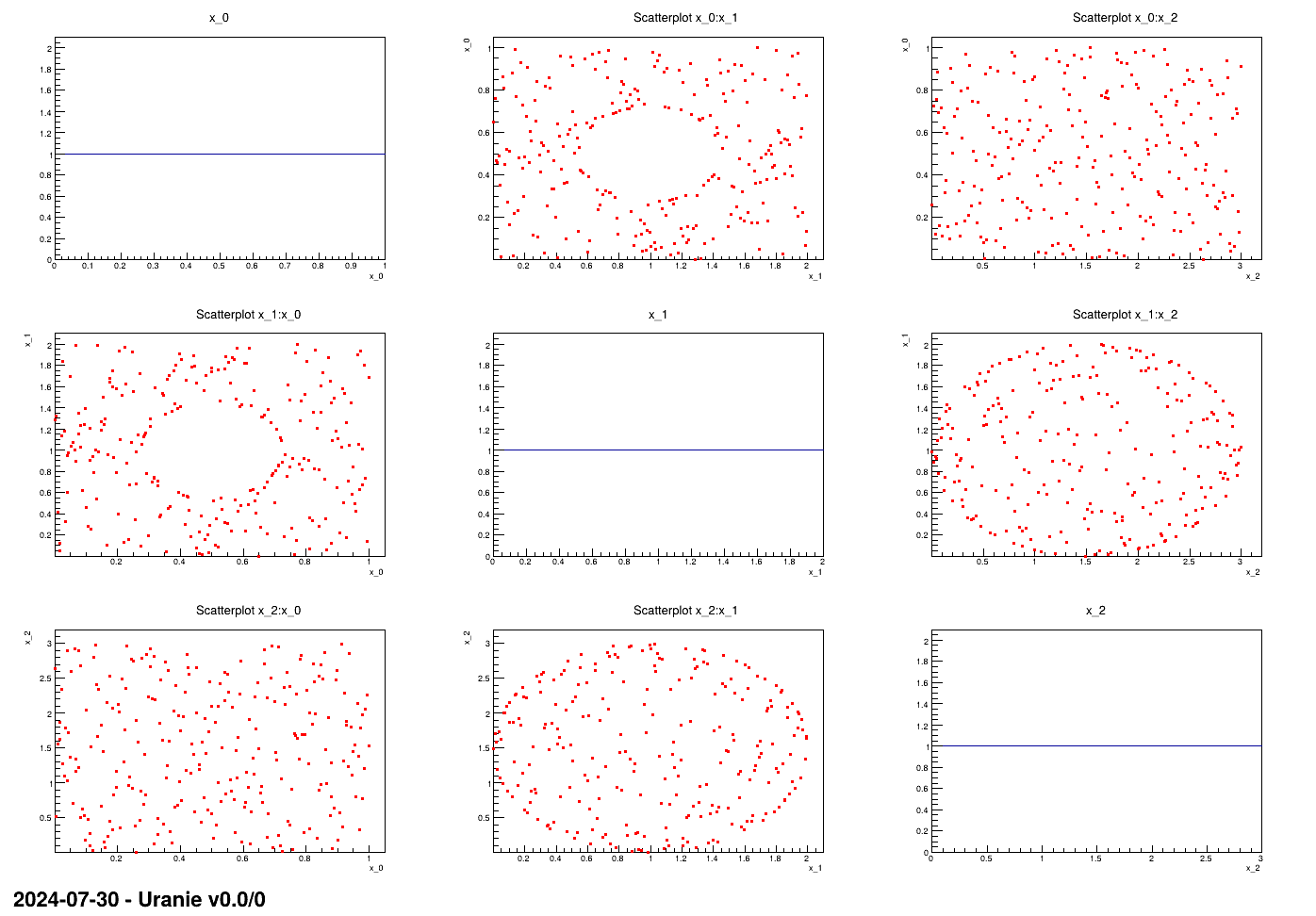
This macro shows the usage of the TConstrLHS class when one wants to create a constrained LHS with non-linear constraints. In order to illustate the concept, it is applied on three input variables drawn from uniform distribution with well-thought boundaries (as the concept of the LHS is to have nicely distributed marginals). The constraints are excluding the inner part of an ellipse for one of the input plane and the outter part of another ellipse for another input plane.

"""
Example of Constrained lhs with ellipses
"""
import numpy as np
from rootlogon import ROOT, DataServer, Sampler


def nicegrid(l_tds, l_can):
    """Generate the grid plot."""

    l_ns = l_tds.getNPatterns()
    l_nx = l_tds.getNAttributes()
    l_tds.drawPairs()

    all_h = []
    ROOT.gStyle.SetOptStat(0)
    for iatt in range(l_nx):
        l_can.GetPad(iatt*(l_nx+1)+1).cd()
        att = l_tds.getAttribute(iatt)
        a_name = att.GetName()
        all_h.append(ROOT.TH1F(a_name+"_histo", a_name+";x_"+str(iatt),
                               l_ns, att.getLowerBound(), att.getUpperBound()))
        l_tds.Draw(a_name+">>"+a_name+"_histo", "", "goff")
        all_h[iatt].Draw()

    return all_h


# Canvas to produce the pair plot
Can = ROOT.TCanvas("Can", "Can", 10, 32, 1400, 1000)
apad = ROOT.TPad("apad", "apad", 0, 0.03, 1, 1)
apad.Draw()
apad.cd()

ns = 250  # Size of the samples to be produced
nx = 3

# Create dataserver and define the attributes
tds = DataServer.TDataServer("tds", "pouet")
for i in range(nx):

    tds.addAttribute(DataServer.TUniformDistribution("x_"+str(i), 0, i+1))
    tds.getAttribute("x_"+str(i)).delShare()

ROOT.gROOT.LoadMacro("ConstrFunctions.C")

# Generate the constr lhs
constrlhs = Sampler.TConstrLHS(tds, ns)
inputs = np.array([1, 0, 1, 2], dtype='i')
constrlhs.addConstraint(ROOT.CircularRules, 2, len(inputs), inputs)
constrlhs.generateSample()

# Do the plot
ListOfDiag = nicegrid(tds, apad)

The very beginning of these macros is the nicegrid method which is here only to show the nice marginal distributions and the scatter plots. One can clearly skip this part to focus on the rest in the main function.

The macro very much looks like any other design-of-experiments generating macro above: the dataserver is created along with the canvas object and the problem is defined along with the input variables and the number of locations to be produced. Once done, then the TConstrLHS instance is created with the four following lines:

# Generate the constr lhs
constrlhs = Sampler.TConstrLHS(tds, ns)
inputs = np.array([1, 0, 1, 2], dtype= i )
constrlhs.addConstraint(ROOT.CircularRules, 2, len(inputs), inputs)
constrlhs.generateSample()

The constructor is pretty obvious, as it takes only the dataserver object and the number of locations. Once created the main method to be called is the addConstraint function which has been largely discussed in Section III.2.4. The first argument of this method is the pointer to the C++ function which has been included in our macro through the line used right before the sampler creation:

ROOT.gROOT.LoadMacro("ConstrFunctions.C")

which contains the CircularRules function. The rest of the argument are the number of constraints, the size of the list of parameters and its content. Finally the nicegrid method is called to produce the nice plot shown in Figure XIV.16

This macro shows the usage of the SVD decomposition for the specific case where the target correlation matrix is singular. The idea is to provide a tool that will allow the user to compare quickly both the TSampling and TBasicSampling implementation, with a singular correlation matrix, or not. In order to do that, a toy random correlation matrix generator is provided.

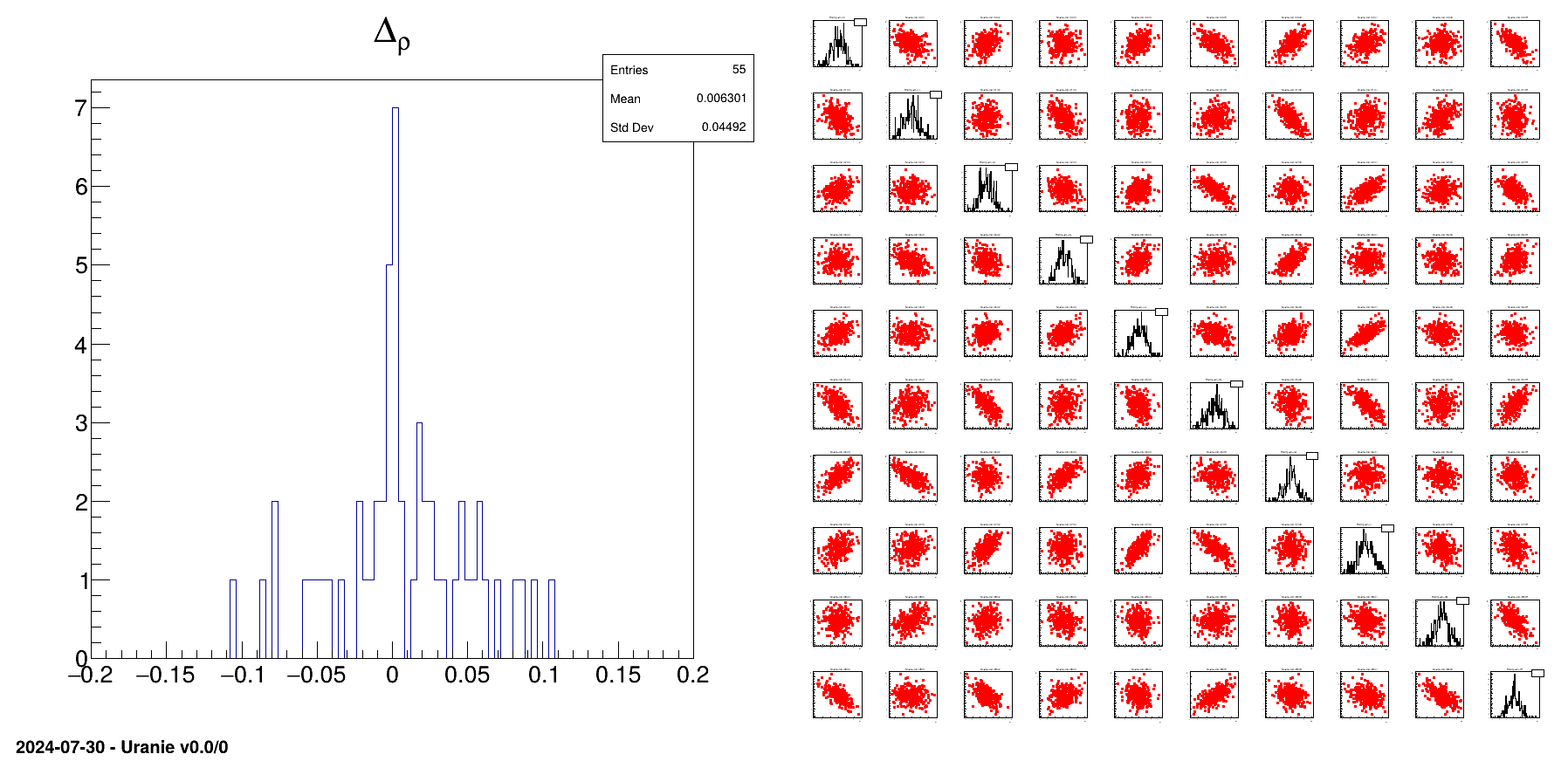
The resulting design-of-experiments is presented side-by-side with the residual of the obtained correlation matrix.

"""
Example of DoE generation when the correlation matrix is singular
"""
from math import sqrt
from rootlogon import ROOT, DataServer, Sampler

# What classes to be used (true==TSampling, false==TBasicSampling)
ImanConover = False
SamplingType = "srs"
# Remove svd to use Cholesky
SamplerOption = "svd"

# Generating randomly a singular correlation matrix
# dimension of the  problem in total.
n = 10
# Number of dimension self explained.
# SHOULD BE SMALLER (singular) OR EQUAL TO (full-rank) n.
p = 6
# number of location in the doe
m = 300

# =======================================================================
#           Internal recipe to get this correlation matrix
# =======================================================================
A = ROOT.TMatrixD(n, p)
Rand = ROOT.TRandom3()
for i in range(n):
    for j in range(p):
        A[i][j] = Rand.Gaus(0., 1.)

Gamma = ROOT.TMatrixD(n, n)
Gamma.MultT(A, A)
Gamma *= 1./n

Sig = ROOT.TMatrixD(n, n)
for i in range(n):
    Sig[i][i] = 1./sqrt(Gamma[i][i])

Corr = ROOT.TMatrixD(Sig, ROOT.TMatrix.kMult, Gamma)
Corr *= Sig
# =======================================================================
#                    Corr is our correlation matrix.
# =======================================================================


# Creating the TDS
tds = DataServer.TDataServer("pouet", "pouet")

# Adding attributes
for i in range(n):
    tds.addAttribute(DataServer.TNormalDistribution("n"+str(i), 0., 1.))

# Create the sampler and generate the doe
if ImanConover:
    sam = Sampler.TSampling(tds, SamplingType, m)
    sam.setCorrelationMatrix(Corr)
    sam.generateSample(SamplerOption)
else:
    sam = Sampler.TBasicSampling(tds, SamplingType, m)
    sam.setCorrelationMatrix(Corr)
    sam.generateCorrSample(SamplerOption)

# Compute the empirical correlation matrix
ResultCorr = tds.computeCorrelationMatrix()
# Change it into a residual matrix
ResultCorr -= Corr

ROOT.gStyle.SetOptStat(1110)
# Plot the results
c = ROOT.TCanvas("c", "c", 1800, 900)
apad = ROOT.TPad("apad", "apad", 0, 0.03, 1, 1)
apad.Draw()
apad.cd()
apad.Divide(2, 1)
apad.cd(1)
# Residual distribution
h = ROOT.TH1F("h", "#Delta_{#rho}", 100, -0.2, 0.2)
for i in range(n):
    for j in range(i, n):
        h.Fill(ResultCorr[i][j])
h.Draw()

# all variables
apad.cd(2)
tds.drawPairs()

This macro starts by a bunch of variables provided to offer many possible configuration, among which:

This is the main part of this macro

## What classes to be used (true==TSampling, false==TBasicSampling)
ImanConover=False 
SamplingType="srs"
## Remove svd to use Cholesky
SamplerOption="svd" 

## Generating randomly a singular correlation matrix
# dimension of the  problem in total.
n = 10; 
## Number of dimension self explained.
## SHOULD BE SMALLER (singular) OR EQUAL TO (full-rank) n.
p = 6; 
# number of location in the doe
m=300; 

Once this is settled, the correlation matrix is created and the dataserver is created and n centered-reduced normal attributes are added. The chosen design-of-experiments is generated with the chosen options:

## Create the sampler and generate the doe
if ImanConover :
    sam = Sampler.TSampling(tds,SamplingType,m); 
    sam.setCorrelationMatrix(Corr);
    sam.generateSample(SamplerOption);
    pass
else :
    sam = Sampler.TBasicSampling(tds,SamplingType,m); 
    sam.setCorrelationMatrix(Corr);
    sam.generateCorrSample(SamplerOption);
    pass

Finally the obtained design-of-experiments is shown along with the residual of all the correlation coefficients (difference between the target values and the obtained ones). This is shown in Figure XIV.17 and can be used to compare the performance of the samplers.