13.6.6. Macro “sensitivityMorrisFunctionFlowrate.py”

13.6.6.1. Objective

The objective of this macro is to perform a Morris sensitivity analysis on a set of eight parameters used in the flowrateModel model described in Presentation of the problem.

13.6.6.2. Macro Uranie

"""
Example of Morris estimation on flowrate
"""
from URANIE import DataServer, Sensitivity
import ROOT

ROOT.gROOT.LoadMacro("UserFunctions.C")

# Define the DataServer
tds = DataServer.TDataServer("tdsflowreate", "DataBase flowreate")

tds.addAttribute(DataServer.TUniformDistribution("rw", 0.05, 0.15))
tds.addAttribute(DataServer.TUniformDistribution("r", 100.0, 50000.0))
tds.addAttribute(DataServer.TUniformDistribution("tu", 63070.0, 115600.0))
tds.addAttribute(DataServer.TUniformDistribution("tl", 63.1, 116.0))
tds.addAttribute(DataServer.TUniformDistribution("hu", 990.0, 1110.0))
tds.addAttribute(DataServer.TUniformDistribution("hl", 700.0, 820.0))
tds.addAttribute(DataServer.TUniformDistribution("l", 1120.0, 1680.0))
tds.addAttribute(DataServer.TUniformDistribution("kw", 9855.0, 12045.0))

nreplique = 3
nlevel = 10
scmo = Sensitivity.TMorris(tds, "flowrateModel", nreplique, nlevel)
scmo.setDrawProgressBar(False)
scmo.generateSample()

tds.exportData("_morris_sampling_.dat")
scmo.computeIndexes()

tds.exportData("_morris_launching_.dat")

ntresu = scmo.getMorrisResults()
ntresu.Scan("*")

# Graph
canmoralltraj = ROOT.gROOT.FindObject("canmoralltraj")
can = ROOT.TCanvas("c1", "Graph of sensitivityMorrisFunctionFlowrate",
                   5, 64, 1270, 667)
pad = ROOT.TPad("pad", "pad", 0, 0.03, 1, 1)
pad.Draw()
pad.Divide(2)
pad.cd(1)
scmo.drawSample("", -1, "nonewcanv")
pad.cd(2)
scmo.drawIndexes("mustar", "", "nonewcanv")

The function flowrateModel is loaded from the macro UserFunctions.C (the file can be found in ${URANIESYS}/share/uranie/macros)

ROOT.gROOT.LoadMacro("UserFunctions.C")

Each parameter is related to the TDataServer as a TAttribute and obeys an uniform law on specific interval:

tds = DataServer.TDataServer("tdsflowreate", "DataBase flowreate")
tds.addAttribute(DataServer.TUniformDistribution("rw", 0.05, 0.15))
tds.addAttribute(DataServer.TUniformDistribution("r", 100.0, 50000.0))
tds.addAttribute(DataServer.TUniformDistribution("tu", 63070.0, 115600.0))
tds.addAttribute(DataServer.TUniformDistribution("tl", 63.1, 116.0))
tds.addAttribute(DataServer.TUniformDistribution("hu", 990.0, 1110.0))
tds.addAttribute(DataServer.TUniformDistribution("hl", 700.0, 820.0))
tds.addAttribute(DataServer.TUniformDistribution("l", 1120.0, 1680.0))
tds.addAttribute(DataServer.TUniformDistribution("kw", 9855.0, 12045.0))

To instantiate the TMorris, one uses the TDataServer, the name of the function, the number of replicas (here nreplique=3), the level parameter (here nlevel=10)

scmo = Sensitivity.TMorris(tds, "flowrateModel", nreplique, nlevel)

Creation of the sampling:

scmo.generateSample()

Data are exported in an ASCII file:

tds.exportData("_morris_sampling_.dat")

Computation of sensitivity indexes:

scmo.computeIndexes()

13.6.6.3. Graph

../../_images/sensitivityMorrisFunctionFlowrate.png — Figure 13.22 Graph of the macro **“sensitivityMorrisFunctionFlowrate.py”**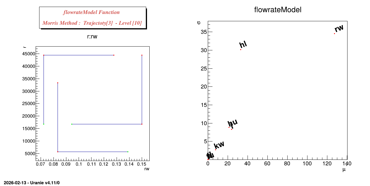

13.6.6.4. Console

************************************************************************
*    Row   *     Input *    Output *     mu.mu * mustar.mu * sigma.sig *
************************************************************************
*        0 *        rw * flowrateM * 127.47900 * 127.47900 * 34.521839 *
*        1 *         r * flowrateM * -0.069601 * 0.0696013 * 0.0793689 *
*        2 *        tu * flowrateM * 0.0004201 * 0.0004201 * 0.0004641 *
*        3 *        tl * flowrateM * 0.4659763 * 0.4659763 * 0.3301256 *
*        4 *        hu * flowrateM * 21.192361 * 21.192361 * 8.8498989 *
*        5 *        hl * flowrateM * -32.74887 * 32.748874 * 30.146134 *
*        6 *         l * flowrateM * -23.89328 * 23.893280 * 8.2781934 *
*        7 *        kw * flowrateM * 7.5766167 * 7.5766167 * 2.7457665 *
************************************************************************