

Documentation
/ Guide méthodologique
: 
| Chapter V. Sensitivity analysis | ||
|---|---|---|
 |  | |
Abstract
This part is introducing the different methods proposed in Uranie to deal with sensitivity analysis. It starts with a very general introduction of simple hypothesis and how to verify them, before discussing more refined strategy, relying for example, on the functional decomposition of the variance.
Table of Contents
In this section, we will briefly remind the different ways to measure the sensitivity of an output to the inputs of the
model. A theoretical introduction will give a glimpse of
different techniques and formalism, going from the simplest case to the more complex one. It should remain at a very
basic level, only to introduce notions since more details can be found in many references
[Salt04,Salt08primer,Salt08].
The list of methods available in Uranie will also be
briefly discussed, as most of these procedures, local and global ones, are further discussed in the following sections
(both implementation and cost in terms of number of assessments).
In this section, the tested hypothesis is to know whether the output of our considered model,  , can be written as a linear approximation, as
follows
, can be written as a linear approximation, as
follows
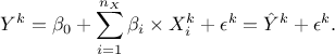
In this equation,  are the linear regression coefficients,
  is the dimension of the input variables,
 is the index of the considered
event in the complete set of data (of size
is the index of the considered
event in the complete set of data (of size  ). In the second equality,
  is the estimation and
  is the regression residual of the k-Th output when using the linear model. In
order to study this case, few numerical expressions can be computed:
is the regression residual of the k-Th output when using the linear model. In
order to study this case, few numerical expressions can be computed:
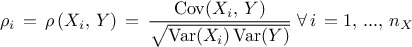
The linear correlation coefficient: also named Pearson coefficient, it is computed as
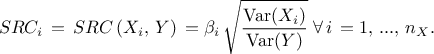
The standard regression coefficient: also named SRC coefficient, it is computed as
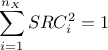
In the case where the various inputs are independent, it is possible to link two of these coefficients by the following relation:
 . Assuming a pure linear model, meaning that
Equation V.1 can be written
. Assuming a pure linear model, meaning that
Equation V.1 can be written  (or equivalently
  ), there is then a closing relation, as follows:
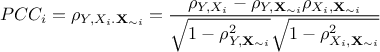
The partial correlation coefficient: also named PCC coefficient. It is defined to quantify the unique sensitivity of the output to
 that cannot be explained in terms of the relations of these variables with
any other variables (i.e. considering that the other variables are constant). It is so
defined as
that cannot be explained in terms of the relations of these variables with
any other variables (i.e. considering that the other variables are constant). It is so
defined as where
 is the vector of input where the i-Th component
has been taken out.
is the vector of input where the i-Th component
has been taken out.
The SRC and PCC coefficients are not equal one to another but they can both be used to sort the inputs according to
their impact on the output, giving the same ranking even though their values would be different. The validity of
the assumption made to consider the model as linear can also be tested by computing "quality criteria". There are
few of them available in Uranie ( ,
,  and
and  )
which have already been discussed in Section IV.1.1.
)
which have already been discussed in Section IV.1.1.
The linearity is a very strong hypothesis, which is rarely correct when dealing with real problems. In order to
circumvent this hypothesis, it is possible to use the ranks (instead of the values) in order to test only the
monotony of the output with respect to the inputs. Each simulation (whose index goes from 1 to ) is ranked according to a variable, 1 being attributed to the simulation
with the lowest value, while
is allocated to the largest one (or the other way around, this should not change the results). It is then
possible, using these ranks instead of the values, to redefine all the previously-discussed expressions:
The correlation coefficient: using the ranks, it is defined like the Pearson coefficient and is called Spearmann coefficient
The standardised regression rank coefficient: using the rank, it is defined like the SRC and is called the SRRC coefficient
The partial rank correlation coefficient: using the rank, it is defined like the PCC and is called the PRCC coefficient


The quality criteria discussed previously in the context of values study, can as well be computed with the ranks. These quality criteria (defined in Section IV.1.1) remain indeed valid to judge the validity of the monotony hypothesis once the same replacement is performed.
When no hypothesis is made on the relation between the inputs and the outputs, one can try a more general
approach. If we can consider that the inputs are independent one to another, it is possible to study how
the output variance diminish when fixing to a certain value  . This variance denoted by
 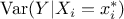 is called the conditional variance and depends on the chosen value
of . In order to study this
dependence, one should consider
is called the conditional variance and depends on the chosen value
of . In order to study this
dependence, one should consider  , the conditional variance over all possible value. It is a random variable and, as
such, one can define the expectation of this quantity as
, the conditional variance over all possible value. It is a random variable and, as
such, one can define the expectation of this quantity as 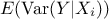 . The value of this newly defined random variable
() is as
small as the impact of on
the output variance is large.
. The value of this newly defined random variable
() is as
small as the impact of on
the output variance is large.
From there it is possible to use the theorem of the total variance which states, under the assumption of having
and two jointly distributed (discrete or continuous)
random variables, that  It becomes clear that the variance of the
conditional expectation can be a good estimator of the sensitivity of the output to the specific input
. It is then more common and
practical to refer to a normalised index in order to define this sensitivity, which is done by writing
It becomes clear that the variance of the
conditional expectation can be a good estimator of the sensitivity of the output to the specific input
. It is then more common and
practical to refer to a normalised index in order to define this sensitivity, which is done by writing
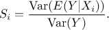
This normalised index is often called the
first order sensitivity index and is, in the specific case of a purely linear theory, equal to
the corresponding SRC coefficient.
If the previously defined index is the first order, then it means that there are higher-order
indices that one might be able to compute. This index which does indeed describe the impact of the input
on the output, does not take
into account the possible interaction between inputs. It can then be completed with the crossed impact of this
particular input with any other  (for
(for  and
and  ). This second order index
  does not take into account the crossed impact of inputs
  and
and  with another one, named for instance (for
  and
and  )... This shows the necessity to consider the
interaction between all the inputs, even though they are not correlated, leading to a set of
)... This shows the necessity to consider the
interaction between all the inputs, even though they are not correlated, leading to a set of  indices to compute. A complete
estimation of all these coefficients is possible and would lead to a perfect break down of the output variance,
which has been proposed by many authors in the literature and is referred to with many names, such as functional
decomposition, ANOVA method (ANalysis Of VAriance), HDMR (High-Dimensional Model
Representation), Sobol's decomposition, Hoeffding's decomposition... This decomposition assumes that
the input factors are independent.
indices to compute. A complete
estimation of all these coefficients is possible and would lead to a perfect break down of the output variance,
which has been proposed by many authors in the literature and is referred to with many names, such as functional
decomposition, ANOVA method (ANalysis Of VAriance), HDMR (High-Dimensional Model
Representation), Sobol's decomposition, Hoeffding's decomposition... This decomposition assumes that
the input factors are independent.
In order to simplify this, it is possible to estimate, for an input , the total order sensitivity index  defined as the sum over all the
sensitivity indices involving the input variable under study [Homma96]:
defined as the sum over all the
sensitivity indices involving the input variable under study [Homma96]:
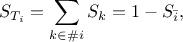
where  and
and  represents respectively the group of indices that contains and
that does not contain the
index. There are few ways to check but also interpret the value of the Sobol sensitivity indices:
represents respectively the group of indices that contains and
that does not contain the
index. There are few ways to check but also interpret the value of the Sobol sensitivity indices:
 :
should always be true.
:
should always be true.
 : the model is purely additive, or in other words, there are no interaction between the
inputs and
: the model is purely additive, or in other words, there are no interaction between the
inputs and  .
.
 is an
indicator of the presence of interactions.
is an
indicator of the presence of interactions.
 is a
direct estimate of the interaction of the i-Th input with all the other factors.
is a
direct estimate of the interaction of the i-Th input with all the other factors.
In Uranie, there are several methods implemented to get both the first order and the total order index of sensitivity and they will be discussed in the upcoming sections.
The decomposition discussed in Section V.1.1.3 and the resulting interpretation in terms of first and total order Sobol indices both suffer from theoretical limitation that are discussed within this section. There are different methods and indices that are said to overcome part of all of the listed issues. This part introduces the limitation and gives an insight of the way to overcome them.
There are few main concerns when dealing with sensitivity indices within the Sobol framework:
there are two indices for every input variables.
On the one hand, first order indices might be obtained but because of their definition their value can be small or even null even though their real impact should not be discarded.
On the other hand, total order indices are very useful to complete the picture provided by the first order ones but they are usually quite costly to obtain and not so many methods can allow to reach them.
the input variables must be independent.
It means input variables must be independant one to another.
It implies, to remain simple, that the inputs and outputs should remain scalars and if not, they should be no correlation between their elements.
Concerning the first observation, the sub-item is right disreagarding the situation: because of its definition based on the evolution of the mean of the conditional output, an input can be discarded even though it has a strong impact as long as the average impact is constant. As soon as one gets the total index (if possible), it completes the picture but having two indices can still be confusing (to understand their meaning). A way to overcome this would be to get another metric providing only one index per variable. The litterature is snowed under with new index definitions in order to overcome these limitations: based on different research field and on various mathematical techniques, one can find such names as HSIC [da2015global], Shapley's values [owen2014sobol], Johnson's relative weights [johnson2000heuristic]...
For the second observation, changing the strategy is also a solution. One possibility is to gather the dependent inputs into a group and only considerer and compare the resulting groups. There will be no hierarchy information within every groups, but this technique will work only if all variables are not dependent. If not, then, rather than relying on a variance decomposition-based technique, one should use other indices once again to overcome this issue. Some methods are discussed later on, in dedicated part, while the rest of this section will briefly introduce the Shapley's values.
The Shapley analysis has originated from the game theory, when considering the case of a coalitional game,
i.e. a couple  where
where
 is the number of players;
 is a function from
 so that
  and
and 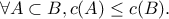 It is called the
characteristic function.
It is called the
characteristic function.
The function has the following
meaning: if  is a coalition of
players, then
is a coalition of
players, then  , called the
worth of coalition , describes
the total expected sum of payoffs the members of can obtain through cooperation. The Shapley's method is one way to distribute the total gains to
the players, assuming that they all collaborate. It is a "fair" distribution in the sense that it is the only
distribution with certain desirable properties listed below. According to the Shapley value, the amount that player
will receive, in a coalitional
game , is
, called the
worth of coalition , describes
the total expected sum of payoffs the members of can obtain through cooperation. The Shapley's method is one way to distribute the total gains to
the players, assuming that they all collaborate. It is a "fair" distribution in the sense that it is the only
distribution with certain desirable properties listed below. According to the Shapley value, the amount that player
will receive, in a coalitional
game , is
The main properties of the Shapley values are the following ones:
efficiency:
symmetry: if
and
are two equivalent
players, meaning  then
then 
additivity: when two coalition games
and  are combined, it defines a new game
  where
where  , then
 .
.
nullity:
 for a null player. A player is null if
The concept of Shapley value has been extensively used in finance for some times but has only recently been brought
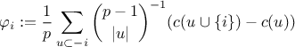
up in the uncertainty community, one can indeed define the Shapley value for a given input , as done in Owen [owen2014sobol]:
where  is the set
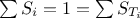
 . Based on this definition, Shapley values have been exhibited as proper sensitivity indices in
[iooss2017shapley] when the inputs are dependent. There is indeed only one value for each input
variable, this value always lies in
. Based on this definition, Shapley values have been exhibited as proper sensitivity indices in
[iooss2017shapley] when the inputs are dependent. There is indeed only one value for each input
variable, this value always lies in  and their sum equals to one, once all input variables are considered (even with correlation).
In the case where  , assuming
  , for the sake of simplicity, without genericity loss, one can rewrite the
sensitivity indices, as they can be calculated explicitly. The Sobol indices, for instance, can be expressed with
expectations of conditional variances [broto2019sensitivity], as done below:
, for the sake of simplicity, without genericity loss, one can rewrite the
sensitivity indices, as they can be calculated explicitly. The Sobol indices, for instance, can be expressed with
expectations of conditional variances [broto2019sensitivity], as done below:
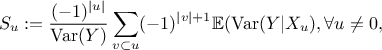
which leads to a new expression for the i-Th Shapley value:
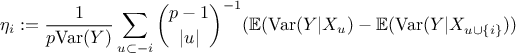
Using the Gaussian framework, one can express the conditional variance as shown here:

This expression is constant for a given subset , so it is equal to its expectation which provide a way to compute all Shapley values.
Methods for Sensitivity Analysis (SA) are split into two types:
- local: variations around a nominal value,
- global: variations in all the domain.
Finite differences (local method):
It consists in estimating the partial derivatives around a nominal value for each input parameters (see Section V.2).
Values Regression method (linearity):
It performs a sensitivity analysis based on the coefficients of a normalised linear regression (see Section V.3).
Ranks Regression method (monotony):
Here, the analysis is based on the coefficients of a normalised rank regression (see Section V.3).
Morris' screening method:
It consists in ordering the input variables according to their influence on the output variables. This method should be used for input ranking. Despite the low computational cost encountered, the obtained information is insufficient to get a proper quantitave estimation of the impact of the input variable on the output under consideration (see Section V.4).
Sobol method:
This method produces numerical values for the Sobol indices. However, it requires a high numerical cost as numerous code assessments are needed (see Section V.5).
It is based on the so-called Saltelli & Tarontola method, to compute the first and total order indices, using different algorithms.
FAST method:
It computes Sobol's first order indices from Fourier coefficients, using a sample on a periodic curve with different frequencies for each input variables (see Section V.6).
RBD method:
It computes Sobol's first order indices from Fourier coefficients, using a sample on a periodic curve with an unique frequency (see Section V.6).
Johnson's relative weights method:
It computes the relative weights which are aimed to be a good approximation of the Shapley's values, but whose main advantage is to be a lot quicker to estimate. This method is limited to linear cases (see Section V.7).
| | | |
| IV.5. The kriging method |  | V.2. The finite differences method |